105 : Nonlinear Poisson Equation
This examples solves the nonlinear Poisson problem
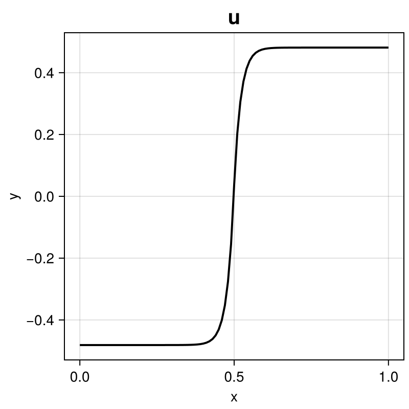
\[\begin{aligned} - \epsilon \partial^2 u / \partial x^2 + e^u - e^{-u} & = f && \text{in } \Omega \end{aligned}\]
where
\[f(x) = \begin{cases} 1 & x \geq 0.5, -1 & x < 0.5. \end{cases}\]
on the domain $\Omega := (0,1)$ with Dirichlet boundary conditions $u(0) = 0$ and $u(1) = 1$.
The solution looks like this:
module Example105_NonlinearPoissonEquation

using ExtendableFEM
using ExtendableGrids

# rigt-hand side data
function f!(result, qpinfo)
	result[1] = qpinfo.x[1] < 0.5 ? -1 : 1
end
# boundary data
function boundary_data!(result, qpinfo)
	result[1] = qpinfo.x[1]
end

# kernel for the (nonlinear) reaction-convection-diffusion oeprator
function nonlinear_kernel!(result, input, qpinfo)
	u, ∇u, ϵ = input[1], input[2], qpinfo.params[1]
	result[1] = exp(u) - exp(-u)
	result[2] = ϵ * ∇u
end

# everything is wrapped in a main function
function main(; Plotter = nothing, h = 1e-2, ϵ = 1e-3, order = 2, kwargs...)

	# problem description
	PD = ProblemDescription("Nonlinear Poisson Equation")
	u = Unknown("u"; name = "u")
	assign_unknown!(PD, u)
	assign_operator!(PD, NonlinearOperator(nonlinear_kernel!, [id(u), grad(u)]; params = [ϵ], kwargs...))
	assign_operator!(PD, LinearOperator(f!, [id(u)]; store = true, kwargs...))
	assign_operator!(PD, InterpolateBoundaryData(u, boundary_data!; kwargs...))

	# discretize: grid + FE space
	xgrid = simplexgrid(0:h:1)
	FES = FESpace{H1Pk{1, 1, order}}(xgrid)

	# generate a solution vector and solve
	sol = solve(PD, FES; kwargs...)

	# plot discrete and exact solution (on finer grid)
	plt = plot([id(u)], sol; Plotter = Plotter)

	return sol, plt
end

end
This page was generated using Literate.jl.