205 : Heat equation
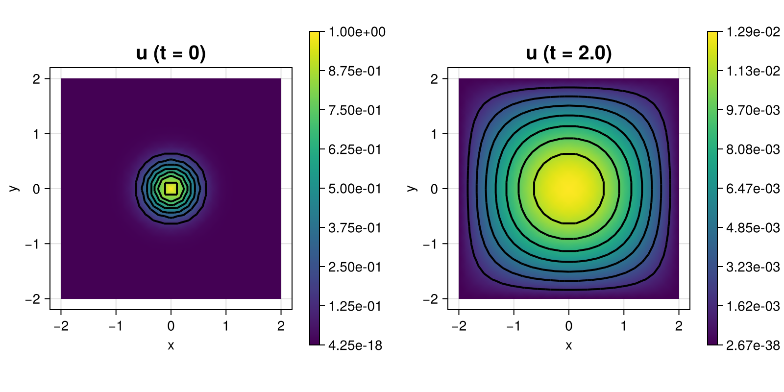
This example computes the solution $u$ of the two-dimensional heat equation
\[\begin{aligned} u_t - \Delta u & = 0 \quad \text{in } \Omega \end{aligned}\]
for homogeneous Dirichlet boundary conditions and some given initial state on the unit square domain $\Omega$ on a given grid.
The initial condition and the final solution for the default parameters looks like this:
module Example205_HeatEquation

using ExtendableFEM
using ExtendableGrids
using DifferentialEquations

# initial state u at time t0
function initial_data!(result, qpinfo)
	x = qpinfo.x
	result[1] = exp(-5 * x[1]^2 - 5 * x[2]^2)
end

function main(; nrefs = 4, T = 2.0, τ = 1e-3, order = 2, use_diffeq = true,
	solver = ImplicitEuler(autodiff = false), Plotter = nothing, kwargs...)

	# problem description
	PD = ProblemDescription("Heat Equation")
	u = Unknown("u")
	assign_unknown!(PD, u)
	assign_operator!(PD, BilinearOperator([grad(u)]; store = true, kwargs...))
	assign_operator!(PD, HomogeneousBoundaryData(u; regions = 1:4))

	# grid
	xgrid = uniform_refine(grid_unitsquare(Triangle2D; scale = [4, 4], shift = [-0.5, -0.5]), nrefs)

	# prepare solution vector and initial data u0
	FES = FESpace{H1Pk{1, 2, order}}(xgrid)
	sol = FEVector(FES; tags = PD.unknowns)
	interpolate!(sol[u], initial_data!; bonus_quadorder = 5)

	# init plotter and plot u0
	plt = plot([id(u)], sol; add = 1, Plotter = Plotter, title_add = " (t = 0)")

	if (use_diffeq)
		# generate DifferentialEquations.ODEProblem
		prob = generate_ODEProblem(PD, FES, (0.0, T); init = sol, constant_matrix = true)

		# solve ODE problem
		de_sol = DifferentialEquations.solve(prob, solver, abstol = 1e-6, reltol = 1e-3, dt = τ, dtmin = 1e-6, adaptive = true)
		@info "#tsteps = $(length(de_sol))"

		# get final solution
		sol.entries .= de_sol[end]
	else
		# add backward Euler time derivative
		M = FEMatrix(FES)
		assemble!(M, BilinearOperator([id(1)]))
		assign_operator!(PD, BilinearOperator(M, [u]; factor = 1 / τ, kwargs...))
		assign_operator!(PD, LinearOperator(M, [u], [u]; factor = 1 / τ, kwargs...))

		# generate solver configuration
		SC = SolverConfiguration(PD, FES; init = sol, maxiterations = 1, constant_matrix = true, kwargs...)

		# iterate tspan
		t = 0
		for it ∈ 1:Int(floor(T / τ))
			t += τ
			ExtendableFEM.solve(PD, FES, SC; time = t)
		end
	end

	# plot final state
	plot!(plt, [id(u)], sol; keep = 1, title_add = " (t = $T)")

	return sol, plt
end

end # module
This page was generated using Literate.jl.