252 : Navier–Stokes Planar Lattice Flow
This example computes an approximation to the planar lattice flow test problem of the Navier-Stokes equations
\[\begin{aligned} - \nu \Delta \mathbf{u} + (\mathbf{u} \cdot \nabla) \mathbf{u} + \nabla p & = \mathbf{f}\\ \mathrm{div}(\mathbf{u}) & = 0 \end{aligned}\]
with an exterior force $\mathbf{f}$ and some viscosity parameter $\nu$ and Dirichlet boundary data for $\mathbf{u}$.
Here the exact data for the planar lattice flow
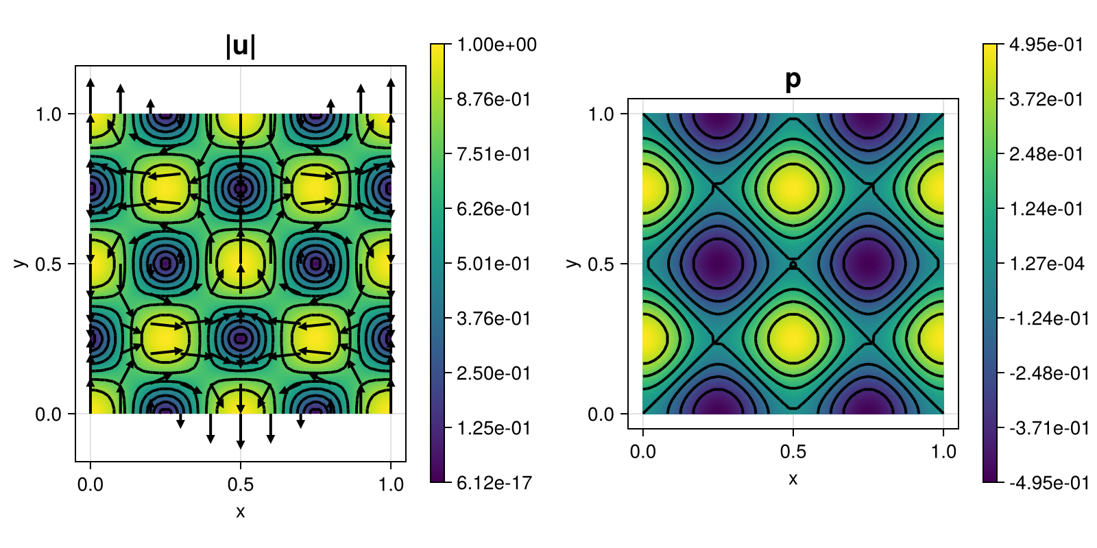
\[\begin{aligned} \mathbf{u}(x,y,t) & := \exp(-8 \pi^2 \nu t) \begin{pmatrix} \sin(2 \pi x) \sin(2 \pi y) \\ \cos(2 \pi x) \cos(2 \pi y) \end{pmatrix}\\ p(x,y,t) & := \exp(-8 \pi^2 \nu t) ( \cos(4 \pi x) - \cos(4 \pi y)) / 4 \end{aligned}\]
is prescribed at fixed time $t = 0$ with $\mathbf{f} = - \nu \Delta \mathbf{u}$.
In this example the Navier-Stokes equations are solved with a pressure-robust variant of the Bernardi–Raugel finite element method and the nonlinear convection term (that involves reconstruction operators) is automatically differentiated for a Newton iteration.
The computed solution for the default parameters looks like this:
module Example252_NSEPlanarLatticeFlow

using ExtendableFEM
using ExtendableGrids
using LinearAlgebra

# exact velocity (and Dirichlet data)
function u!(result, qpinfo)
	x = qpinfo.x
	result[1] = sin(2 * pi * x[1]) * sin(2 * pi * x[2])
	result[2] = cos(2 * pi * x[1]) * cos(2 * pi * x[2])
end

# right-hand side f := -μ Δu + (u⋅∇)u + ∇p
function f!(μ)
	α = [0, 0]
	function closure(result, qpinfo)
		x = qpinfo.x
		result[1] = (μ * 8 * pi^2 + α[1]) * sin(2 * pi * x[1]) * sin(2 * pi * x[2])
		result[2] = (μ * 8 * pi^2 + α[2]) * cos(2 * pi * x[1]) * cos(2 * pi * x[2])
	end
end

# exact pressure
function p!(result, qpinfo)
	x = qpinfo.x
	result[1] = (cos(4 * pi * x[1]) - cos(4 * pi * x[2])) / 4
end

function kernel_nonlinear!(result, u_ops, qpinfo)
	u, ∇u, p = view(u_ops, 1:2), view(u_ops, 3:6), view(u_ops, 7)
	μ = qpinfo.params[1]
	result[1] = dot(u, view(∇u, 1:2))
	result[2] = dot(u, view(∇u, 3:4))
	result[3] = μ * ∇u[1] - p[1]
	result[4] = μ * ∇u[2]
	result[5] = μ * ∇u[3]
	result[6] = μ * ∇u[4] - p[1]
	result[7] = -(∇u[1] + ∇u[4])
	return nothing
end

function exact_error!(result, u, qpinfo)
	u!(result, qpinfo)
	p!(view(result, 3), qpinfo)
	result .-= u
	result .= result .^ 2
end

function main(; μ = 0.001, nrefs = 5, reconstruct = true, Plotter = nothing, kwargs...)

	# problem description
	PD = ProblemDescription()
	u = Unknown("u"; name = "velocity")
	p = Unknown("p"; name = "pressure")
	id_u = reconstruct ? apply(u, Reconstruct{HDIVBDM1{2}, Identity}) : id(u)

	assign_unknown!(PD, u)
	assign_unknown!(PD, p)
	assign_operator!(PD, NonlinearOperator(kernel_nonlinear!, [id_u, grad(u), id(p)]; params = [μ], kwargs...))
	assign_operator!(PD, LinearOperator(f!(μ), [id_u]; kwargs...))
	assign_operator!(PD, InterpolateBoundaryData(u, u!; regions = 1:4))

	# grid
	xgrid = uniform_refine(grid_unitsquare(Triangle2D), nrefs)

	# prepare FESpace
	FES = [FESpace{H1BR{2}}(xgrid), FESpace{L2P0{1}}(xgrid)]

	# solve
	sol = solve(PD, FES; kwargs...)

	# move integral mean of pressure
	pintegrate = ItemIntegrator([id(p)])
	pmean = sum(evaluate(pintegrate, sol)) / sum(xgrid[CellVolumes])
	view(sol[p]) .-= pmean

	# error calculation
	ErrorIntegratorExact = ItemIntegrator(exact_error!, [id(u), id(p)]; quadorder = 4, params = [μ], kwargs...)
	error = evaluate(ErrorIntegratorExact, sol)
	L2errorU = sqrt(sum(view(error, 1, :)) + sum(view(error, 2, :)))
	L2errorP = sqrt(sum(view(error, 3, :)))
	@info "L2error(u) = $L2errorU"
	@info "L2error(p) = $L2errorP"

	# plot
	plt = plot([id(u), id(p)], sol; Plotter = Plotter)

	return L2errorU, plt
end

end # module
This page was generated using Literate.jl.