282 : Incompressible MHD
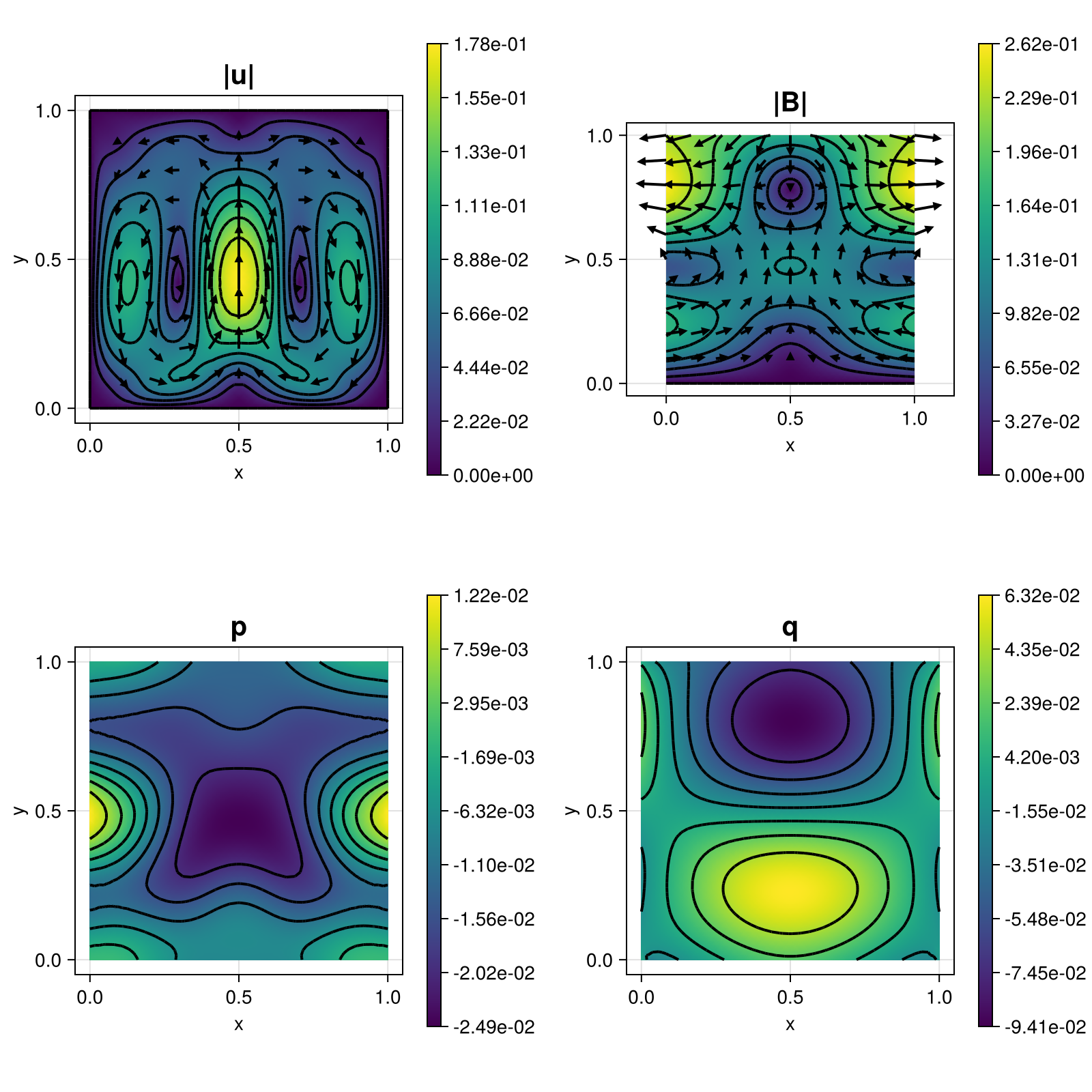
This example yields a prototype for te stationary incompressible viscious MHD equations that seek a velocity field $\mathbf{u}$, a pressure field $p$ and a divergence-free magnetic field $\mathbf{B}$ such that
\[\begin{aligned} - \mu \Delta \mathbf{u} + \nabla \cdot (\mathbf{u} \otimes \mathbf{u} - \mathbf{B} \otimes \mathbf{B}) + \nabla (p + \frac{1}{2} \mathbf{B} \cdot \mathbf{B}) & = 0\\ \mathrm{div}(\mathbf{u}) & = 0\\ - \eta \Delta \mathbf{B} + \nabla \cdot (\mathbf{u} \otimes \mathbf{B} - \mathbf{B} \otimes \mathbf{u}) & = 0\\ \mathrm{div}(\mathbf{B}) & = 0\\ \end{aligned}\]
on a rectangular 2D domain. Here, $\mu$ and $\eta$ are the viscosity and resistivity of the fluid and the magnetic field, respectively.
module Example282_IncompressibleMHD

using ExtendableFEM
using ExtendableGrids
using LinearAlgebra

function f!(result, qpinfo)
	result .= 0
end

function g!(result, qpinfo)
	x = qpinfo.x
	result[1] = sin(2*pi*x[2])*cos(pi*x[1])
	result[2] = 0
end

function kernel_nonlinear!(result, u_ops, qpinfo)
    u, B, ∇u, ∇B, p, q = view(u_ops, 1:2), view(u_ops, 3:4), view(u_ops, 5:8), view(u_ops, 9:12), view(u_ops, 13), view(u_ops, 14)
	μ = qpinfo.params[1]
    η = qpinfo.params[2]

	# viscous terms and pressures
    result[5] = μ * ∇u[1] - p[1]
	result[6] = μ * ∇u[2]
	result[7] = μ * ∇u[3]
	result[8] = μ * ∇u[4] - p[1]
	result[9] = η * ∇B[1] - q[1]
	result[10] = η * ∇B[2]
	result[11] = η * ∇B[3]
	result[12] = η * ∇B[4] - q[1]

    # Lorentz force
    result[1] = - dot(B, view(∇B,1:2))
    result[2] = - dot(B, view(∇B,3:4))
    BdotB = (B[1]*B[1] + B[2]*B[2])/2
    result[5] -= BdotB
    result[8] -= BdotB

    # convection term for u and B
	result[1] += dot(u, view(∇u,1:2))
	result[2] += dot(u, view(∇u,3:4))
	result[3] = dot(u, view(∇B,1:2)) - dot(B, view(∇u,1:2))
	result[4] = dot(u, view(∇B,3:4)) - dot(B, view(∇u,3:4))

    # divergence constraint
	result[13] = -(∇u[1] + ∇u[4])
	result[14] = -(∇B[1] + ∇B[4])
	return nothing
end


# everything is wrapped in a main function
function main(; Plotter = nothing, μ = 1e-3, η = 1e-1, nrefs = 5, kwargs...)

	# load grid (see function below)
	xgrid = uniform_refine(grid_unitsquare(Triangle2D), nrefs)

	# problem description
	PD = ProblemDescription()
	u = Unknown("u"; name = "velocity")
	B = Unknown("B"; name = "magnetic field")
	p = Unknown("p"; name = "pressure")
	q = Unknown("q"; name = "magnetic pressure")

	assign_unknown!(PD, u)
	assign_unknown!(PD, B)
	assign_unknown!(PD, p)
	assign_unknown!(PD, q)

    assign_operator!(PD, NonlinearOperator(kernel_nonlinear!, [id(u), id(B), grad(u), grad(B), id(p), id(q)]; bonus_quadorder = 2, params = [μ,η], kwargs...))
    assign_operator!(PD, LinearOperator(f!, [id(u)]))
    assign_operator!(PD, LinearOperator(g!, [id(B)]))
    assign_operator!(PD, HomogeneousBoundaryData(u; regions = 1:4))
    assign_operator!(PD, HomogeneousBoundaryData(B; regions = [1]))
    assign_operator!(PD, FixDofs(p; dofs = [1]))
    assign_operator!(PD, FixDofs(q; dofs = [1]))

	# P2-bubble finite element method
	FETypes = [H1P2{2, 2}, H1P2{2, 2}, H1P1{1}, H1P1{1}]

	# generate FESpaces and Solution vector
	FES = [FESpace{FETypes[j]}(xgrid) for j = 1:4]

	# solve
    sol = ExtendableFEM.solve(PD, FES; target_residual = 1e-8, time = 0, kwargs...)

    # plot
	plt = plot([id(u), id(B), id(p), id(q)], sol; Plotter = Plotter)

	return sol, plt
end

end
This page was generated using Literate.jl.