204 : Eigenvalue problem for the Laplacian
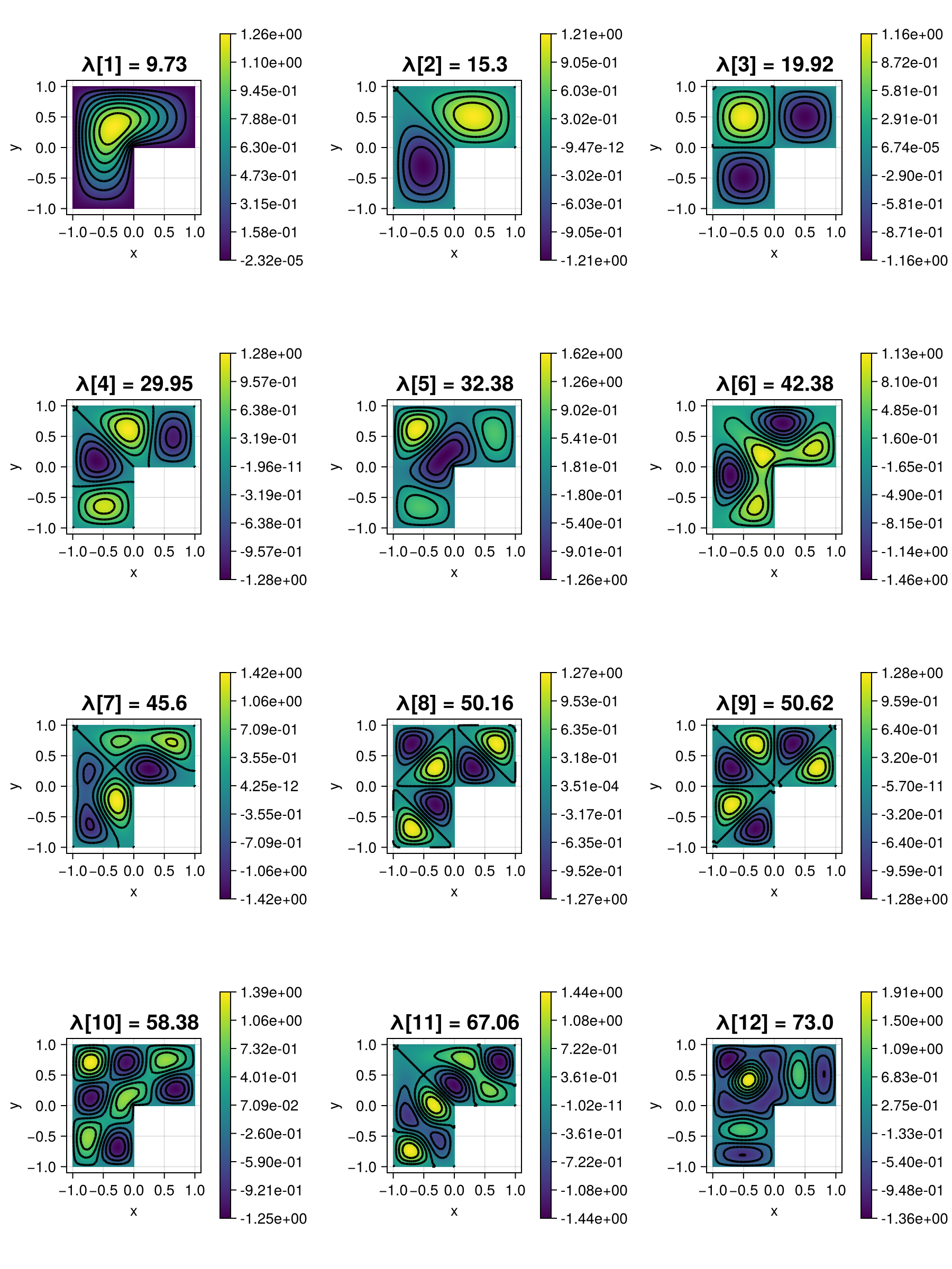
This example computes the pairs of eigenvalues and eigenvectors $(\lambda,u) \in \mathbb{R} \times H^1_0(\Omega)$ of the Laplacian, i.e,
\[\begin{aligned} -\Delta u & = \lambda u \quad \text{in } \Omega \end{aligned}\]
on a two-dimensional L-shaped domain with homogeneous boundary conditions with the help of an iterative solver from KrylovKit.jl. The first twelve computed eigenvectors look like this:
module Example204_LaplaceEVProblem

using ExtendableFEM
using ExtendableGrids
using ExtendableSparse
using LinearAlgebra
using GridVisualize
using KrylovKit

function main(; which = 1:12, ncols = 3, nrefs = 4, order = 1, Plotter = nothing, kwargs...)

	# discretize
	xgrid = uniform_refine(grid_lshape(Triangle2D), nrefs)
	FES = FESpace{H1Pk{1, 2, order}}(xgrid)

	# assemble operators
	A = FEMatrix(FES)
	B = FEMatrix(FES)
	u = FEVector(FES; name = "u")
	assemble!(A, BilinearOperator([grad(1)]; kwargs...))
	assemble!(A, BilinearOperator([id(1)]; entities = ON_BFACES, factor = 1e4, kwargs...))
	assemble!(B, BilinearOperator([id(1)]; kwargs...))

	# solver generalized eigenvalue problem iteratively with KrylovKit
	λs, x, info = geneigsolve((A.entries, B.entries), maximum(which), :SR; maxiter = 4000, issymmetric = true, tol = 1e-8)
	@show info
	@assert info.converged >= maximum(which)

	# plot requested eigenvalue pairs
	nEVs = length(which)
	nrows = Int(ceil(nEVs / ncols))
	plt = GridVisualizer(; Plotter = Plotter, layout = (nrows, ncols), clear = true, resolution = (900, 900 / ncols * nrows))
	col, row = 0, 1
	for j in which
		col += 1
		if col == ncols + 1
			col, row = 1, row + 1
		end
		λ = λs[j]
		@info "λ[$j] = $λ, residual = $(sum(info.residual[j]))"
		u.entries .= Real.(x[j])
		scalarplot!(plt[row, col], id(1), u; Plotter = Plotter, title = "λ[$j] = $(Float16(λ))")
	end

	return u, plt
end

end # module
This page was generated using Literate.jl.