284 : Level Set Method
This example studies the level-set method of some level function $\mathbf{\phi}$ convected in time via the equation
\[\begin{aligned} \phi_t + \mathbf{u} \cdot \nabla \phi & = 0. \end{aligned}\]
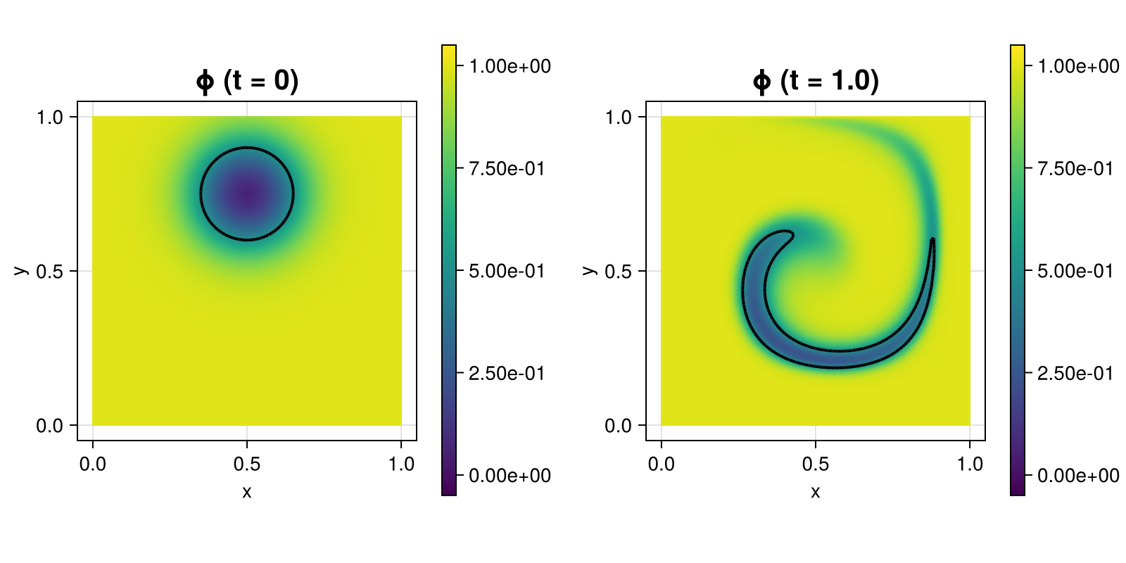
Here this is tested with the (conservative) initial level set function $\phi(x) = 0.5 \tanh((\lvert x - (0.25,0.25) \rvert - 0.1)/(2ϵ) + 1)$ such that the level $\phi \equiv 0.5$ forms a circle which is then convected by the velocity $\mathbf{u} = (0.5,1)^T$. No reinitialisation step is performed.
The initial condition and the final solution for the default parameters looks like this:
module Example284_LevelSetMethod

using ExtendableFEM
using ExtendableGrids
using GridVisualize
using DifferentialEquations

function ϕ_init!(result, qpinfo)
	x = qpinfo.x
	ϵ = qpinfo.params[1]
	result[1] = 1 / 2 * (tanh((sqrt((x[1] - 0.25)^2 + (x[2] - 0.25)^2) - 0.1) / (2 * ϵ)) + 1)
end

function kernel_convection!(result, input, qpinfo)
	result[1] = 0.5 * input[1] + input[2]
end

# everything is wrapped in a main function
function main(; Plotter = nothing, ϵ = 0.05, τ = 1e-3, T = 0.4, order = 2, nref = 5, use_diffeq = true,
	solver = ImplicitEuler(autodiff = false), kwargs...)

	# initial grid and final time
	xgrid = uniform_refine(grid_unitsquare(Triangle2D), nref)

	# define main level set problem
	PD = ProblemDescription("level set problem")
	ϕ = Unknown("ϕ"; name = "level set function")
	assign_unknown!(PD, ϕ)
	assign_operator!(PD, BilinearOperator(kernel_convection!, [id(ϕ)], [grad(ϕ)]; kwargs...))
	assign_operator!(PD, HomogeneousBoundaryData(ϕ; value = 1, regions = 1:4, kwargs...))

	# generate FESpace and solution vector and interpolate initial state
	FES = FESpace{H1Pk{1, 2, order}}(xgrid)
	sol = FEVector(FES; tags = PD.unknowns)
	interpolate!(sol[ϕ], ϕ_init!; params = [ϵ])

	# prepare plot and plot init solution
	plt = GridVisualizer(; Plotter = Plotter, layout = (1, 2), clear = true, resolution = (800, 400))
	scalarplot!(plt[1, 1], id(ϕ), sol; levels = [0.5], flimits = [-0.05, 1.05], colorbarticks = [0, 0.25, 0.5, 0.75, 1], title = "ϕ (t = 0)")

	if (use_diffeq)
		# generate DifferentialEquations.ODEProblem
		prob = generate_ODEProblem(PD, FES, (0.0, T); init = sol, constant_matrix = true)

		# solve ODE problem
		de_sol = DifferentialEquations.solve(prob, solver, abstol = 1e-6, reltol = 1e-4, dt = τ, dtmin = 1e-8, adaptive = true)
		@info "#tsteps = $(length(de_sol))"

		# get final solution
		sol.entries .= de_sol[end]
	else
		# add backward Euler time derivative
		M = FEMatrix(FES)
		assemble!(M, BilinearOperator([id(1)]))
		assign_operator!(PD, BilinearOperator(M, [ϕ]; factor = 1 / τ, kwargs...))
		assign_operator!(PD, LinearOperator(M, [ϕ], [ϕ]; factor = 1 / τ, kwargs...))

		# generate solver configuration
		SC = SolverConfiguration(PD, FES; init = sol, maxiterations = 1, constant_matrix = true, kwargs...)

		# iterate tspan
		t = 0
		for it ∈ 1:Int(floor(T / τ))
			t += τ
			ExtendableFEM.solve(PD, FES, SC; time = t)
		end
	end

	# plot final state
	scalarplot!(plt[1, 2], id(ϕ), sol; levels = [0.5], flimits = [-0.05, 1.05], colorbarticks = [0, 0.25, 0.5, 0.75, 1], title = "ϕ (t = $T)")

	return sol, plt
end

end
This page was generated using Literate.jl.