270 : Natural convection

(source code)

Seek velocity $\mathbf{u}$, pressure $p$ and temperature $\theta$ such that

\[\begin{aligned} - \mu \Delta u + (\mathbf{u} \cdot \nabla) \mathbf{u} + \nabla p & = Ra \, \theta \, g \\ - \Delta \theta + \mathbf{u} \cdot \nabla \theta & = 0 \end{aligned}\]

on a given domain $\Omega$ (here a triangle) and boundary conditions

\[\begin{aligned} \mathbf{u} & = 0 && \quad \text{along } \partial \Omega\\ T & = T_\text{bottom} &&\quad \text{along } y = 0\\ T & = 0 &&\quad \text{along } x = 0 \end{aligned}\]

The weak formulation seeks $(\mathbf{u},p,\theta) \in V \times Q \times X \subseteq H^1_0(\Omega)^2 \times L^2_0(\Omega) \times H^1_D(\Omega)$ such that

\[\begin{aligned} (\mu \nabla \mathbf{u}, \nabla \mathbf{v}) + ((\mathbf{u} \cdot \nabla) \mathbf{u}, \mathbf{v}) - (\mathrm{div} \mathbf{v}, p) & = (\mathbf{v}, Ra g \, \theta) && \quad \text{for all } \mathbf{v} \in V,\\ (\mathrm{div} \mathbf{u}, q) & = 0 && \quad \text{for all } q \in Q,\\ (\nabla \theta, \nabla \varphi) + (u \cdot \nabla \theta, \varphi) & = 0 && \quad \text{for all } \varphi \in X. \end{aligned}\]

To render the discrete method pressure-robust, a reconstruction operator is applied to all identity evaluations of $\mathbf{u}$ and $\mathbf{v}$ (when the switch reconstruct is set to true). Further explanations and discussion on this example can be found in the reference below.

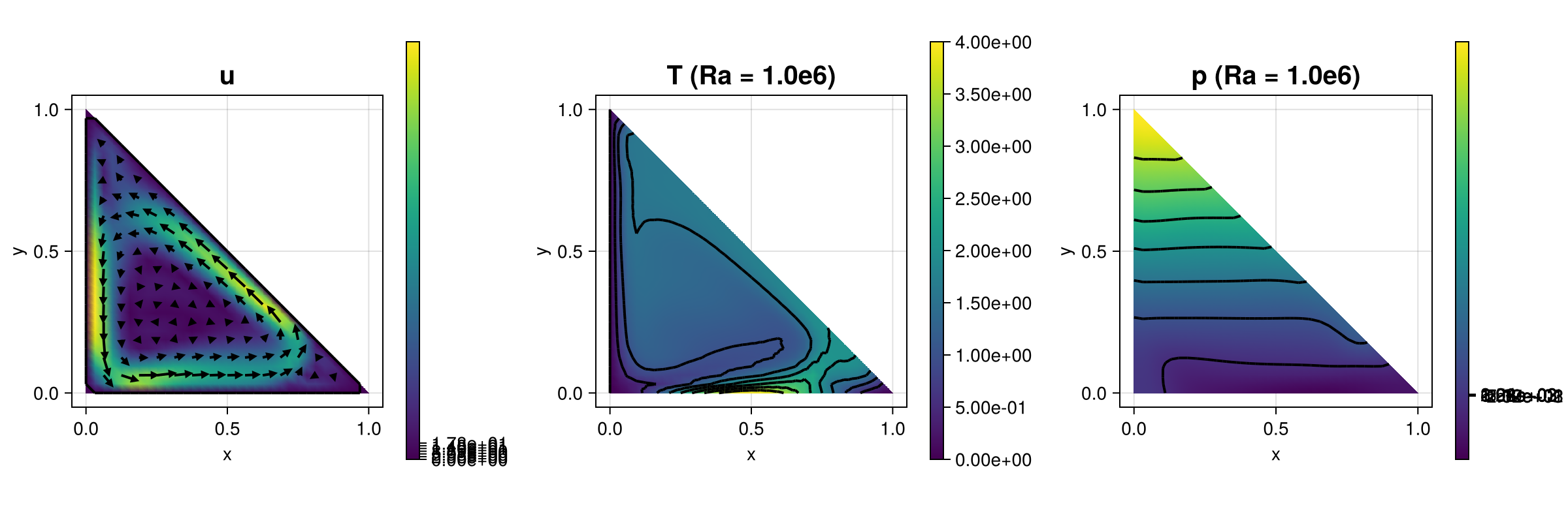
The computed solution for the default parameters looks like this:

module Example270_NaturalConvectionProblem

using ExtendableFEM
using ExtendableGrids
using GridVisualize
using LinearAlgebra

function kernel_nonlinear!(result, u_ops, qpinfo)
    u, ∇u, p, ∇T, T = view(u_ops, 1:2), view(u_ops,3:6), view(u_ops, 7), view(u_ops, 8:9), view(u_ops, 10)
    Ra, μ, ϵ = qpinfo.params[1], qpinfo.params[2], qpinfo.params[3]
    result[1] = dot(u, view(∇u,1:2))
    result[2] = dot(u, view(∇u,3:4)) - Ra*T[1]
    result[3] = μ*∇u[1] - p[1]
    result[4] = μ*∇u[2]
    result[5] = μ*∇u[3]
    result[6] = μ*∇u[4] - p[1]
    result[7] = -(∇u[1] + ∇u[4])
    result[8] = ϵ*∇T[1]
    result[9] = ϵ*∇T[2]
    result[10] = dot(u, ∇T)
    return nothing
end

function T_bottom!(result, qpinfo)
    x = qpinfo.x
    result[1] = 2*(1-cos(2*π*x[1]))
end

function main(;
    nrefs = 5,
    μ = 1.0,
    ϵ = 1.0,
    Ra_final = 1.0e6,
    reconstruct = true,
    Plotter = nothing,
    kwargs...)

    # problem description
    PD = ProblemDescription()
    u = Unknown("u"; name = "velocity")
    p = Unknown("p"; name = "pressure")
    T = Unknown("T"; name = "temperature")
    assign_unknown!(PD, u)
    assign_unknown!(PD, p)
    assign_unknown!(PD, T)
    id_u = reconstruct ? apply(u, Reconstruct{HDIVBDM1{2}, Identity}) : id(u)
    assign_operator!(PD, NonlinearOperator(kernel_nonlinear!, [id_u,grad(u),id(p),grad(T),id(T)]; kwargs...))
    assign_operator!(PD, HomogeneousBoundaryData(u; regions = 1:3))
    assign_operator!(PD, FixDofs(p; dofs = [1], vals = [0]))
    assign_operator!(PD, HomogeneousBoundaryData(T; regions = 3))
    assign_operator!(PD, InterpolateBoundaryData(T, T_bottom!; regions = 1))

    # grid
    xgrid = uniform_refine(reference_domain(Triangle2D), nrefs)

    # FESpaces
    FES = Dict(u => FESpace{H1BR{2}}(xgrid),
               p => FESpace{L2P0{1}}(xgrid),
               T => FESpace{H1P1{1}}(xgrid))

    # prepare plots
    plt = GridVisualizer(; Plotter = Plotter, layout = (1,3), clear = true, size = (1200,400))

    # solve by Ra embedding
	params = Array{Float64,1}([min(Ra_final, 4000), μ, ϵ])
    sol = nothing
    SC = nothing
	step = 0
	while (true)
        # solve (params are given to all operators)
        sol, SC = ExtendableFEM.solve(PD, FES, SC; init = sol, return_config = true, target_residual = 1e-6, params = params, kwargs...)

        # plot
        scalarplot!(plt[1,1], id(u), sol; levels = 0, colorbarticks = 7, abs = true)
        vectorplot!(plt[1,1], id(u), sol; clear = false, title = "|u| + quiver (Ra = $(params[1]))")
        scalarplot!(plt[1,2], id(T), sol; title = "T (Ra = $(params[1]))")
        scalarplot!(plt[1,3], id(p), sol; title = "p (Ra = $(params[1]))")

        # stop if Ra_final is reached
		if params[1] >= Ra_final
			break
		end

        # increase Ra
		params[1] = min(Ra_final, params[1]*3)
		step += 1
		@info "Step $step : solving for Ra=$(params[1])"
	end

    # compute Nusselt number along bottom (= boundary region 1)
    ∇T_faces = FaceInterpolator([jump(grad(T))]; order = 0, kwargs...)
	NuIntegrator = ItemIntegrator((result, input, qpinfo) -> (result[1] = -input[2]), [id(1)]; entities = ON_FACES, regions = [1])
    Nu = sum(evaluate(NuIntegrator, evaluate!(∇T_faces, sol)))
	@info "Nu = $Nu"

    return Nu, plt
end

end # module

This page was generated using Literate.jl.