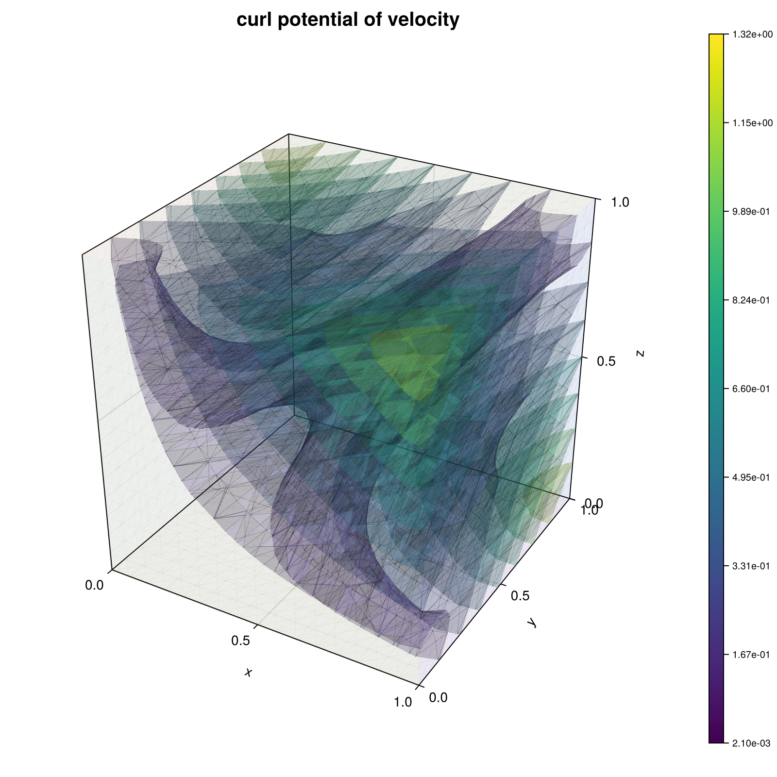
310 : Div-free RT0 basis
This example computes the best-approximation $\mathbf{\psi}_h$ of a divergence-free velocity $\mathbf{u} = \mathrm{curl} \mathbf{\psi}$ by solving for a curl-potential $\mathbf{\phi}_h \in N_0$ with
\[\begin{aligned} (\mathrm{curl} \mathbf{\phi}_h, \mathrm{curl} \mathbf{\theta}_h) & = (\mathbf{u}, \mathrm{curl} \mathbf{\theta}_h) \quad \text{for all } \mathbf{\theta} \in N_0 \end{aligned}\]
Here, $N_0$ denotes the lowest-order Nedelec space which renders the problem ill-posed unless one selects a linear independent basis. This is done with the algorithm suggested in the reference below.
"Decoupling three-dimensional mixed problems using divergence-free finite elements",
R. Scheichl,
SIAM J. Sci. Comput. 23(5) (2002),
>Journal-Link<
The computed solution for the default parameters looks like this:
module Example310_DivFreeBasis

using ExtendableFEM
using GridVisualize
using ExtendableGrids
using ExtendableSparse
using LinearAlgebra
using Symbolics

# exact data for problem generated by symbolics
function prepare_data()

	@variables x y z

	# stream function ξ
	ξ = [x*y*z,x*y*z,x*y*z]

	# velocity u = curl ξ
	∇ξ = Symbolics.jacobian(ξ, [x, y, z])
	u = [∇ξ[3,2] - ∇ξ[2,3], ∇ξ[1,3] - ∇ξ[3,1], ∇ξ[2,1] - ∇ξ[1,2]]

	# build function
	u_eval = build_function(u, x, y, z, expression = Val{false})

	return u_eval[2]
end

function main(;
	nrefs = 4,                      ## number of refinement levels
	bonus_quadorder = 2,            ## additional quadrature order for data evaluations
	divfree_basis = true,			## if true uses curl(N0), if false uses mixed FEM RT0xP0
	Plotter = nothing,              ## Plotter (e.g. PyPlot)
	kwargs...)

	# prepare problem data
	u_eval = prepare_data()
	exact_u!(result, qpinfo) = (u_eval(result, qpinfo.x[1], qpinfo.x[2], qpinfo.x[3]))

	# prepare plots
	plt = GridVisualizer(; Plotter = Plotter, layout = (2, 2), clear = true, size = (800, 800))

	# prepare error calculation
	function exact_error!(result, u, qpinfo)
		exact_u!(view(result, 1:3), qpinfo)
		result .-= u
		result .= result .^ 2
	end
	ErrorIntegratorExact = ItemIntegrator(exact_error!, [divfree_basis ? curl3(1) : id(1)]; bonus_quadorder = 2 + bonus_quadorder, kwargs...)
	NDofs = zeros(Int, nrefs)
	L2error = zeros(Float64, nrefs)

	sol = nothing
	for lvl ∈ 1:nrefs
		# grid
		xgrid = uniform_refine(grid_unitcube(Tetrahedron3D), lvl)

		if divfree_basis

			# use Nedelec FESpace and determine linear independent basis
			FES = FESpace{HCURLN0{3}}(xgrid)

			@time begin
				# get subset of edges, spanning the node graph
				spanning_tree = get_spanning_edge_subset(xgrid)

				# get all other edges = linear independent degrees of freedom
				subset = setdiff(1:num_edges(xgrid), spanning_tree)
			end
			NDofs[lvl] = length(subset)

			# assemble full Nedelec curl-curl problem...
			u = Unknown("u"; name = "curl potential of velocity")
			PD = ProblemDescription("curl-curl formulation")
			assign_unknown!(PD, u)
			assign_operator!(PD, BilinearOperator([curl3(u)]))
			assign_operator!(PD, LinearOperator(exact_u!, [curl3(u)]; bonus_quadorder = bonus_quadorder))

			# ...and solve with subset
			sol = solve(PD, FES; restrict_dofs = [subset[:]])
		else
			# use RT0 functions + side constraint for divergence
			FES = [FESpace{HDIVRT0{3}}(xgrid), FESpace{L2P0{1}}(xgrid)]
			NDofs[lvl] = FES[1].ndofs + FES[2].ndofs

			u = Unknown("u"; name = "velocity")
			p = Unknown("u"; name = "pressure")
			PD = ProblemDescription("mixed formulation")
			assign_unknown!(PD, u)
			assign_unknown!(PD, p)
			assign_operator!(PD, BilinearOperator([id(u)]))
			assign_operator!(PD, BilinearOperator([div(u)], [id(p)]; transposed_copy = 1))
			assign_operator!(PD, LinearOperator(exact_u!, [id(u)]; bonus_quadorder = bonus_quadorder))
			sol = solve(PD, FES)
		end

		# evalute error
		error = evaluate(ErrorIntegratorExact, sol)
		L2error[lvl] = sqrt(sum(view(error, 1, :)) + sum(view(error, 2, :)))
		if divfree_basis
			@info "|| u - curl(ϕ_h) || = $(L2error[lvl])"
		else
			@info "|| u - u_h || = $(L2error[lvl])"
		end
	end

	# plot
	if divfree_basis
		scalarplot!(plt[1, 1], curl3(1), sol; abs = true)
	else
		scalarplot!(plt[1, 1], id(1), sol; abs = true)
	end

	# print convergence history as table
	print_convergencehistory(NDofs, L2error; X_to_h = X -> X .^ (-1 / 3), ylabels = ["|| u - u_h ||"], xlabel = "ndof")

	return L2error, plt
end


# finds a minimal subset (of dimension #nodes - 1) of edges, such that all nodes are connected
function get_spanning_edge_subset(xgrid)
	nnodes = num_nodes(xgrid)
	edgenodes = xgrid[EdgeNodes]
	bedgenodes = xgrid[BEdgeNodes]
	bedgeedges = xgrid[BEdgeEdges]

	# boolean arrays to memorize which nodes are visited
	# and which edges belong to the spanning tree
	visited = zeros(Bool, nnodes)
	markededges = zeros(Bool, num_edges(xgrid))

	function find_spanning_tree(edgenodes, remap)
		nodeedges = atranspose(edgenodes)
		function recursive(node)
			visited[node] = true
			nneighbors = num_targets(nodeedges, node)
			for e = 1 : nneighbors
				edge = nodeedges[e, node]
				for k = 1 : 2
					node2 = edgenodes[k, edge]
					if !visited[node2]
						# mark edge
						markededges[remap[edge]] = true
						recursive(node2)
					end
				end
			end
			return nothing
		end
		recursive(edgenodes[1])
	end

	# find spanning tree for Neumann boundary
	# local bedges >> global edge numbers
	find_spanning_tree(bedgenodes, bedgeedges)

	# find spanning tree for remaining part
	other_nodes = setdiff(1:nnodes, unique(view(bedgenodes,:)))
	if length(other_nodes) > 0
		find_spanning_tree(edgenodes, 1 : num_edges(xgrid))
	end

	# return all marked edges
	return findall(==(true), markededges)
end

end # module
This page was generated using Literate.jl.