250 : Navier–Stokes Lid-driven cavity
This example computes the velocity $\mathbf{u}$ and pressure $\mathbf{p}$ of the incompressible Navier–Stokes problem
\[\begin{aligned} - \mu \Delta \mathbf{u} + \left(\mathbf{u} \cdot \nabla\right) \mathbf{u}+ \nabla p & = \mathbf{f}\\ \mathrm{div}(\mathbf{u}) & = 0 \end{aligned}\]
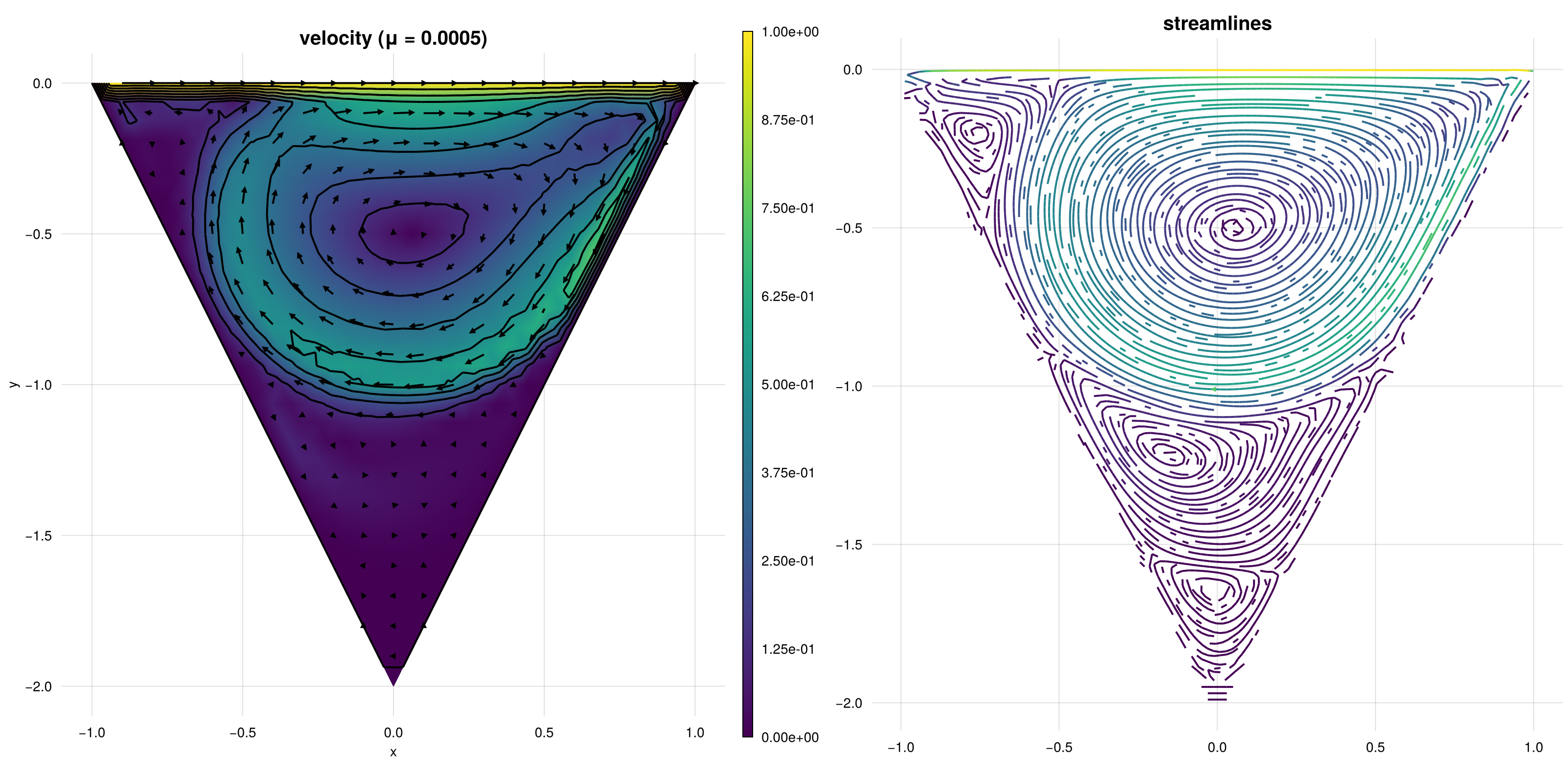
in a lid driven cavity example over a cone and plots the solution and the formed eddies.
The computed solution for the default parameters looks like this:
module Example250_NSELidDrivenCavity

using ExtendableFEM
using GridVisualize
using ExtendableGrids
using LinearAlgebra

function kernel_nonlinear!(result, u_ops, qpinfo)
	u, ∇u, p = view(u_ops, 1:2), view(u_ops, 3:6), view(u_ops, 7)
	μ = qpinfo.params[1]
	result[1] = dot(u, view(∇u, 1:2))
	result[2] = dot(u, view(∇u, 3:4))
	result[3] = μ * ∇u[1] - p[1]
	result[4] = μ * ∇u[2]
	result[5] = μ * ∇u[3]
	result[6] = μ * ∇u[4] - p[1]
	result[7] = -(∇u[1] + ∇u[4])
	return nothing
end

function boundarydata!(result, qpinfo)
	result[1] = 1
	result[2] = 0
end

function initialgrid_cone()
	xgrid = ExtendableGrid{Float64, Int32}()
	xgrid[Coordinates] = Array{Float64, 2}([-1 0; 0 -2; 1 0]')
	xgrid[CellNodes] = Array{Int32, 2}([1 2 3]')
	xgrid[CellGeometries] = VectorOfConstants{ElementGeometries, Int}(Triangle2D, 1)
	xgrid[CellRegions] = ones(Int32, 1)
	xgrid[BFaceRegions] = Array{Int32, 1}([1, 2, 3])
	xgrid[BFaceNodes] = Array{Int32, 2}([1 2; 2 3; 3 1]')
	xgrid[BFaceGeometries] = VectorOfConstants{ElementGeometries, Int}(Edge1D, 3)
	xgrid[CoordinateSystem] = Cartesian2D
	return xgrid
end

function main(; μ_final = 0.0005, order = 2, nrefs = 5, Plotter = nothing, kwargs...)

	# prepare parameter field
	extra_params = Array{Float64, 1}([max(μ_final, 0.05)])

	# problem description
	PD = ProblemDescription()
	u = Unknown("u"; name = "velocity")
	p = Unknown("p"; name = "pressure")

	assign_unknown!(PD, u)
	assign_unknown!(PD, p)
	assign_operator!(PD, NonlinearOperator(kernel_nonlinear!, [id(u), grad(u), id(p)]; params = extra_params, kwargs...))
	assign_operator!(PD, InterpolateBoundaryData(u, boundarydata!; regions = 3))
	assign_operator!(PD, HomogeneousBoundaryData(u; regions = [1, 2]))
	assign_operator!(PD, FixDofs(p; dofs = [1]))


	# grid
	xgrid = uniform_refine(initialgrid_cone(), nrefs)

	# prepare FESpace
	FES = [FESpace{H1Pk{2,2,order}}(xgrid), FESpace{H1Pk{1,2,order-1}}(xgrid)]

	# prepare plots
	plt = GridVisualizer(; Plotter = Plotter, layout = (1, 2), clear = true, size = (1600, 800))

	# solve by μ embedding
	step = 0
	sol = nothing
	SC = nothing
	PE = PointEvaluator([id(1)])
	while (true)
		step += 1
		@info "Step $step : solving for μ=$(extra_params[1])"
		sol, SC = ExtendableFEM.solve(PD, FES, SC; return_config = true, target_residual = 1e-10, maxiterations = 20, kwargs...)
		if step == 1
			initialize!(PE, sol)
		end
		scalarplot!(plt[1, 1], xgrid, nodevalues(sol[1]; abs = true)[1, :]; title = "velocity (μ = $(extra_params[1]))", Plotter = Plotter)
		vectorplot!(plt[1, 1], xgrid, eval_func_bary(PE), spacing = 0.05, clear = false)
		streamplot!(plt[1, 2], xgrid, eval_func_bary(PE), spacing = 0.01, density = 2, title = "streamlines")

		if extra_params[1] <= μ_final
			break
		else
			extra_params[1] = max(μ_final, extra_params[1] / 2)
		end
	end

	scalarplot!(plt[1, 1], xgrid, nodevalues(sol[1]; abs = true)[1, :]; title = "velocity (μ = $(extra_params[1]))", Plotter = Plotter)
	vectorplot!(plt[1, 1], xgrid, eval_func_bary(PE), spacing = 0.05, clear = false)
	streamplot!(plt[1, 2], xgrid, eval_func_bary(PE), spacing = 0.01, density = 2, title = "streamlines")

	return sol, plt
end

end # module
This page was generated using Literate.jl.