108 : Robin Boundary Condition
This demonstrates the assignment of a mixed Robin boundary condition for a nonlinear 1D convection-diffusion-reaction PDE on the unit interval, i.e.
\[\begin{aligned} -\partial^2 u / \partial x^2 + u \partial u / \partial x + u & = f && \text{in } \Omega\\ u + \partial u / \partial_x & = g && \text{at } \Gamma_1 = \{ 0 \}\\ u & = u_D && \text{at } \Gamma_2 = \{ 1 \} \end{aligned}\]
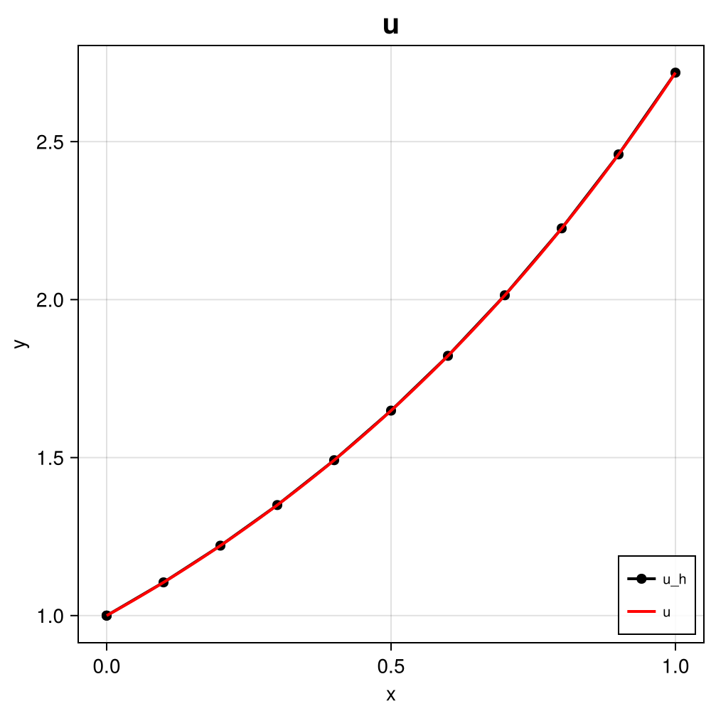
tested with data $f(x) = e^{2x}$, $g = 2$ and $u_D = e$ such that $u(x) = e^x$ is the exact solution.
The solution looks like this:
module Example108_RobinBoundaryCondition

using ExtendableFEM
using ExtendableGrids
using GridVisualize

# data and exact solution
function f!(result, qpinfo)
	result[1] = exp(2 * qpinfo.x[1])
end
function u!(result, qpinfo)
	result[1] = exp(qpinfo.x[1])
end

# kernel for the (nonlinear) reaction-convection-diffusion oeprator
function nonlinear_kernel!(result, input, qpinfo)
	u, ∇u = input[1], input[2]
	result[1] = u * ∇u + u 	# convection + reaction (will be multiplied with v)
	result[2] = ∇u         	# diffusion (will be multiplied with ∇v)
	return nothing
end

# kernel for Robin boundary condition
function robin_kernel!(result, input, qpinfo)
	result[1] = 2 - input[1] # = g - u (will be multiplied with v)
	return nothing
end

# everything is wrapped in a main function
function main(; Plotter = nothing, h = 1e-1, h_fine = 1e-3, order = 2, kwargs...)

	# problem description
	PD = ProblemDescription()
	u = Unknown("u"; name = "u")
	assign_unknown!(PD, u)
	assign_operator!(PD, NonlinearOperator(nonlinear_kernel!, [id(u), grad(u)]; kwargs...))
	assign_operator!(PD, BilinearOperator(robin_kernel!, [id(u)]; entities = ON_BFACES, regions = [1], kwargs...))
	assign_operator!(PD, LinearOperator(f!, [id(u)]; kwargs...))
	assign_operator!(PD, InterpolateBoundaryData(u, u!; regions = [2], kwargs...))

	# generate coarse and fine mesh
	xgrid = simplexgrid(0:h:1)

	# choose finite element type and generate FESpace
	FEType = H1Pk{1, 1, order}
	FES = FESpace{FEType}(xgrid)

	# generate a solution vector and solve
	sol = solve(PD, FES; kwargs...)

	# plot discrete and exact solution (on finer grid)
	plt = GridVisualizer(Plotter = Plotter, layout = (1, 1))
	scalarplot!(plt[1, 1], id(u), sol; color = :black, label = "u_h", markershape = :circle, markersize = 10, markevery = 1)
	xgrid_fine = simplexgrid(0:h_fine:1)
	scalarplot!(plt[1, 1], xgrid_fine, view(nodevalues(xgrid_fine, u!), 1, :), clear = false, color = (1, 0, 0), label = "u", legend = :rb, markershape = :none)

	return sol, plt
end

end
This page was generated using Literate.jl.