106 : Nonlinear Diffusion
This example solves the nonlinear diffusion equation
\[\begin{aligned} u_t - \Delta u^m & = 0 \end{aligned}\]
in $\Omega := (-1,1)$ with homogeneous Neumann boundary conditions.
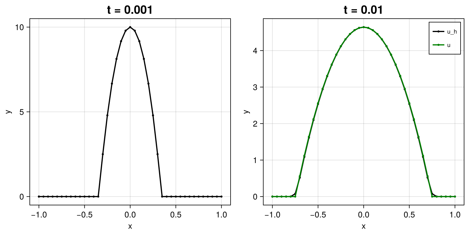
The solution looks like this:
module Example106_NonlinearDiffusion

using ExtendableFEM
using ExtendableGrids
using DifferentialEquations
using GridVisualize

# Barenblatt solution
# (see Barenblatt, G. I. "On nonsteady motions of gas and fluid in porous medium." Appl. Math. and Mech.(PMM) 16.1 (1952): 67-78.)
function u_exact!(result, qpinfo)
	t = qpinfo.time
	x = qpinfo.x[1]
	m = qpinfo.params[1]
	tx = t^(-1.0 / (m + 1.0))
	xx = x * tx
	xx = xx * xx
	xx = 1 - xx * (m - 1) / (2.0 * m * (m + 1))
	if xx < 0.0
		xx = 0.0
	end
	result[1] = tx * xx^(1.0 / (m - 1.0))
end

function kernel_nonlinear!(result, input, qpinfo)
	u, ∇u = input[1], input[2]
	m = qpinfo.params[1]
	result[1] = m * u^(m - 1) * ∇u
end

# everything is wrapped in a main function
function main(;
	m = 2,
	h = 0.05,
	t0 = 0.001,
	T = 0.01,
	order = 1,
	τ = 0.0001,
	Plotter = nothing,
	use_diffeq = true,
	use_masslumping = true,
	solver = ImplicitEuler(autodiff = false),
	kwargs...)

	# load mesh and exact solution
	xgrid = simplexgrid(-1:h:1)

	# set finite element types [surface height, velocity]
	FEType = H1Pk{1, 1, order}

	# generate empty PDEDescription for three unknowns (h, u)
	PD = ProblemDescription("Nonlinear Diffusion Equation")
	u = Unknown("u"; name = "u")
	assign_unknown!(PD, u)
	assign_operator!(PD, NonlinearOperator(kernel_nonlinear!, [grad(u)], [id(u), grad(u)]; params = [m], bonus_quadorder = 2))

	# prepare solution vector and initial data
	FES = FESpace{FEType}(xgrid)
	sol = FEVector(FES; tags = PD.unknowns)
	interpolate!(sol[u], u_exact!; time = t0, params = [m])

	# init plotter and plot u0
	plt = GridVisualizer(; Plotter = Plotter, layout = (1, 2), size = (800,400))
	scalarplot!(plt[1, 1], id(u), sol; label = "u_h", markershape = :circle, markevery = 1, title = "t = $t0")

	# generate mass matrix (with mass lumping)
	M = FEMatrix(FES)
	assemble!(M, BilinearOperator([id(1)]; lump = 2 * use_masslumping))

	if (use_diffeq)
		# generate ODE problem
		prob = ExtendableFEM.generate_ODEProblem(PD, FES, (t0, T); init = sol, mass_matrix = M.entries.cscmatrix)

		# solve ODE problem
		de_sol = DifferentialEquations.solve(prob, solver, abstol = 1e-6, reltol = 1e-3, dt = τ, dtmin = 1e-8, adaptive = true)
		@info "#tsteps = $(length(de_sol))"

		# get final solution
		sol.entries .= de_sol[end]
	else
		# add backward Euler time derivative
		assign_operator!(PD, BilinearOperator(M, [u]; factor = 1 / τ, kwargs...))
		assign_operator!(PD, LinearOperator(M, [u], [u]; factor = 1 / τ, kwargs...))

		# generate solver configuration
		SC = SolverConfiguration(PD, FES; init = sol, maxiterations = 1, kwargs...)

		# iterate tspan
		t = 0
		for it ∈ 1:Int(floor((T - t0) / τ))
			t += τ
			ExtendableFEM.solve(PD, FES, SC; time = t)
		end
	end

	# plot final state and exact solution for comparison
	scalarplot!(plt[1, 2], id(u), sol; label = "u_h", markershape = :circle, markevery = 1)
	interpolate!(sol[1], u_exact!; time = T, params = [m])
	scalarplot!(plt[1, 2], id(u), sol; clear = false, color = :green, label = "u", title = "t = $T", legend = :best)

	return sol, plt
end

end
This page was generated using Literate.jl.