235 : Stokes iterated penalty method

(source code)

This example computes a velocity $\mathbf{u}$ and pressure $\mathbf{p}$ of the incompressible Stokes problem

\[\begin{aligned} - \mu \Delta \mathbf{u} + \nabla p & = \mathbf{0}\\ \mathrm{div}(\mathbf{u}) & = 0 \end{aligned}\]

with some μ parameter $\mu$.

Here we solve the simple Hagen-Poiseuille flow on the two-dimensional unit square domain with the iterated penalty method suggested in the reference below adapted to the Bernardi–Raugel finite element method. Given intermediate solutions $\mathbf{u}_h$ and $p_h$ the next approximations are computed by the two equations

\[\begin{aligned} (\nabla \mathbf{u}_h^{next}, \nabla \mathbf{v}_h) + \lambda (\mathrm{div}_h(\mathbf{u}^{next}_h) ,\mathrm{div}_h(\mathbf{v}_h)) & = (\mathbf{f},\mathbf{v}_h) + (p_h,\mathrm{div}(\mathbf{v}_h)) && \text{for all } \mathbf{v}_h \in \mathbf{V}_h\\ (p^{next}_h,q_h) & = (p_h,q_h) - \lambda (\mathrm{div}(\mathbf{u}_h^{next}),q_h) && \text{for all } q_h \in Q_h \end{aligned}\]

This is done consecutively until the residual of both equations is small enough. The discrete divergence is computed via a RT0 reconstruction operator that preserves the disrete divergence. (another way would be to compute $B M^{-1} B^T$ where $M$ is the mass matrix of the pressure and $B$ is the matrix for the div-pressure block).

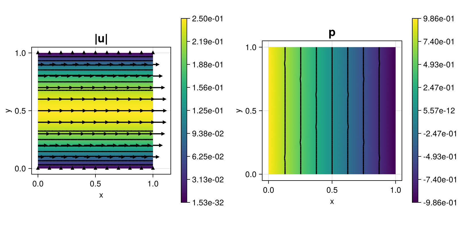
The computed solution for the default parameters looks like this:

module Example235_StokesIteratedPenalty

using ExtendableFEM
using ExtendableGrids

# data for Hagen-Poiseuille flow
function p!(result, qpinfo)
	x = qpinfo.x
	μ = qpinfo.params[1]
	result[1] = μ * (-2 * x[1] + 1.0)
end
function u!(result, qpinfo)
	x = qpinfo.x
	result[1] = x[2] * (1.0 - x[2])
	result[2] = 0.0
end
# kernel for div projection
function div_projection!(result, input, qpinfo)
	result[1] = input[1] - qpinfo.params[1] * input[2]
end

# everything is wrapped in a main function
function main(; Plotter = nothing, λ = 1e4, μ = 1.0, nrefs = 5, kwargs...)

	# initial grid
	xgrid = uniform_refine(grid_unitsquare(Triangle2D), nrefs)

	# Bernardi--Raugel element with reconstruction operator
	FETypes = (H1BR{2}, L2P0{1})
	PenaltyDivergence = Reconstruct{HDIVRT0{2}, Divergence}

	# generate two problems
	# one for velocity, one for pressure
	u = Unknown("u"; name = "velocity")
	p = Unknown("p"; name = "pressure")
	PDu = ProblemDescription("Stokes IPM - velocity update")
	assign_unknown!(PDu, u)
	assign_operator!(PDu, BilinearOperator([grad(u)]; factor = μ, store = true, kwargs...))
	assign_operator!(PDu, BilinearOperator([apply(u, PenaltyDivergence)]; store = true, factor = λ, kwargs...))
	assign_operator!(PDu, LinearOperator([div(u)], [id(p)]; factor = 1, kwargs...))
	assign_operator!(PDu, InterpolateBoundaryData(u, u!; regions = 1:4, params = [μ], bonus_quadorder = 4, kwargs...))

	PDp = ProblemDescription("Stokes IPM - pressure update")
	assign_unknown!(PDp, p)
	assign_operator!(PDp, BilinearOperator([id(p)]; store = true, kwargs...))
	assign_operator!(PDp, LinearOperator(div_projection!, [id(p)], [id(p), div(u)]; params = [λ], factor = 1, kwargs...))

	# show and solve problem
	FES = [FESpace{FETypes[1]}(xgrid), FESpace{FETypes[2]}(xgrid)]
	sol = FEVector([FES[1], FES[2]]; tags = [u, p])
	SC1 = SolverConfiguration(PDu; init = sol, maxiterations = 1, target_residual = 1e-8, constant_matrix = true, kwargs...)
	SC2 = SolverConfiguration(PDp; init = sol, maxiterations = 1, target_residual = 1e-8, constant_matrix = true, kwargs...)
	sol, nits = iterate_until_stationarity([SC1, SC2]; init = sol, kwargs...)
	@info "converged after $nits iterations"

	# plot
	plt = plot([id(u), id(p)], sol; Plotter = Plotter)

	return sol, plt
end

end

This page was generated using Literate.jl.