280 : Compressible Stokes

(source code)

This example solves the two-dimensional compressible Stokes equations where one seeks a (vector-valued) velocity $\mathbf{u}$, a density $\varrho$ and a pressure $p$ such that

\[\begin{aligned} - \mu \Delta \mathbf{u} + \lambda \nabla(\mathrm{div}(\mathbf{u})) + \nabla p & = \mathbf{f} + \varrho \mathbf{g}\\ \mathrm{div}(\varrho \mathbf{u}) & = 0\\ p & = eos(\varrho)\\ \int_\Omega \varrho \, dx & = M\\ \varrho & \geq 0. \end{aligned}\]

Here, eos $eos$ is some equation of state function that describes the dependence of the pressure on the density (and further physical quantities like temperature in a more general setting). Moreover, $\mu$ and $\lambda$ are Lame parameters and $\mathbf{f}$ and $\mathbf{g}$ are given right-hand side data.

There are two testcases. The first testcase solves an analytical toy problem with the prescribed solution

\[\begin{aligned} \mathbf{u}(\mathbf{x}) & =0\\ \varrho(\mathbf{x}) & = \exp(-y/c) \\ p &= eos(\varrho) := c \varrho^\gamma \end{aligned}\]

such that $\mathbf{f} = 0$ and $\mathbf{g}$ nonzero to match the prescribed solution. The second testcase tests an analytical nonzero velocity benchmark problem with the same density.

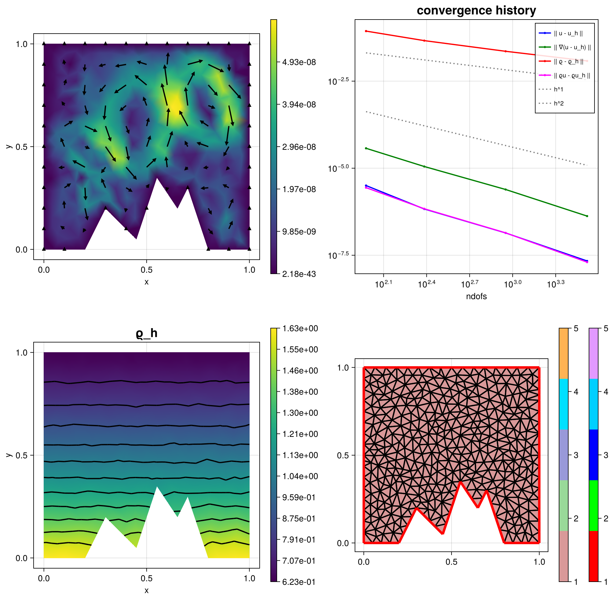
This example is designed to study the well-balanced property of a discretisation. The gradient-robust discretisation approximates the well-balanced state much better, i.e. has a much smaller L2 velocity error. For larger c (= smaller Mach number) the problem gets more incompressible which reduces the error further as then the right-hand side is a perfect gradient also when evaluated with the (now closer to a constant) discrete density. See reference below for more details.

The computed solution for the default parameters looks like this:

module Example280_CompressibleStokes

using ExtendableFEM
using ExtendableGrids
using Triangulate
using SimplexGridFactory
using GridVisualize
using Symbolics
using LinearAlgebra

# everything is wrapped in a main function
# testcase = 1 : well-balanced test (stratified no-flow over mountain)
# testcase = 2 : vortex example (ϱu is div-free p7 vortex)
function main(;
    testcase = 1,
    nrefs = 4,
    M = 1,
    c = 1,
    ufac = 100,
    pressure_stab = 0,
    laplacian_in_rhs = false, # for data in example 2
    maxsteps = 5000,
    target_residual = 1e-11,
    Plotter = nothing,
    reconstruct = true,
    μ = 1,
    order = 1,
    kwargs...)

	# load data for testcase
    grid_builder, kernel_gravity!, kernel_rhs!, u!, ∇u!, ϱ!, τfac = load_testcase_data(testcase; laplacian_in_rhs = laplacian_in_rhs, M = M, c = c, μ = μ, ufac = ufac)
    xgrid = grid_builder(nrefs)

    # define unknowns
    u = Unknown("u"; name = "velocity", dim = 2)
    ϱ = Unknown("ϱ"; name = "density", dim = 1)
    p = Unknown("p"; name = "pressure", dim = 1)

    # define reconstruction operator
    if order == 1
        FETypes = [H1BR{2}, L2P0{1}, L2P0{1}]
        id_u = reconstruct ? apply(u, Reconstruct{HDIVRT0{2}, Identity}) : id(u)
    elseif order == 2
        FETypes = [H1P2B{2,2}, L2P1{1}, L2P1{1}]
        id_u = reconstruct ? apply(u, Reconstruct{HDIVRT1{2}, Identity}) : id(u)
    end

    # define first sub-problem: Stokes equations to solve for velocity u
    PD = ProblemDescription("Stokes problem")
    assign_unknown!(PD, u)
    assign_operator!(PD, BilinearOperator([grad(u)]; factor = μ, store = true, kwargs...))
    assign_operator!(PD, LinearOperator([div(u)], [id(ϱ)]; factor = c, kwargs...))
    assign_operator!(PD, HomogeneousBoundaryData(u; regions = 1:4, kwargs...))
    if kernel_rhs! !== nothing
        assign_operator!(PD, LinearOperator(kernel_rhs!, [id_u]; factor = 1, store = true, bonus_quadorder = 3*order, kwargs...))
    end
    assign_operator!(PD, LinearOperator(kernel_gravity!, [id_u], [id(ϱ)]; factor = 1, bonus_quadorder = 3*order, kwargs...))

    # FVM for continuity equation
	τ = μ / (order^2*M*sqrt(τfac)) # time step for pseudo timestepping
    @info "timestep = $τ"
    PDT = ProblemDescription("continuity equation")
    assign_unknown!(PDT, ϱ)
    if order > 1
       assign_operator!(PDT, BilinearOperator(kernel_continuity!,[grad(ϱ)],[id(ϱ)],[id(u)]; quadorder = 2*order, factor = -1, kwargs...))
    end
    if pressure_stab > 0
        psf = pressure_stab #* xgrid[CellVolumes][1]
        assign_operator!(PDT, BilinearOperator(stab_kernel!, [jump(id(ϱ))], [jump(id(ϱ))], [id(u)]; entities = ON_IFACES, factor = psf, kwargs...))
    end
    assign_operator!(PDT, BilinearOperator([id(ϱ)]; quadorder = 2*(order-1), factor = 1/τ, store = true, kwargs...))
    assign_operator!(PDT, LinearOperator([id(ϱ)], [id(ϱ)]; quadorder = 2*(order-1), factor = 1/τ, kwargs...))
    assign_operator!(PDT, BilinearOperatorDG(kernel_upwind!, [jump(id(ϱ))], [this(id(ϱ)), other(id(ϱ))], [id(u)]; quadorder = order+1, entities = ON_IFACES, kwargs...))

    # prepare error calculation
    EnergyIntegrator = ItemIntegrator(energy_kernel!, [id(u)]; resultdim = 1, quadorder = 2*(order+1), kwargs...)
    ErrorIntegratorExact = ItemIntegrator(exact_error!(u!, ∇u!, ϱ!), [id(u), grad(u), id(ϱ)]; resultdim = 9, quadorder = 2*(order+1), kwargs...)
    NDofs = zeros(Int, nrefs)
    Results = zeros(Float64, nrefs, 5)

    sol = nothing
    xgrid = nothing
    op_upwind = 0
    for lvl = 1 : nrefs
        xgrid = grid_builder(lvl)
        @show xgrid
        FES = [FESpace{FETypes[j]}(xgrid) for j = 1 : 3]
        sol = FEVector(FES; tags = [u,ϱ,p])

        # initial guess
        fill!(sol[ϱ],M)
        interpolate!(sol[u], u!)
        interpolate!(sol[ϱ], ϱ!)
        NDofs[lvl] = length(sol.entries)

        # solve the two problems iteratively [1] >> [2] >> [1] >> [2] ...
        SC1 = SolverConfiguration(PD; init = sol, maxiterations = 1, target_residual = target_residual, constant_matrix = true, kwargs...)
        SC2 = SolverConfiguration(PDT; init = sol, maxiterations = 1, target_residual = target_residual, kwargs...)
        sol, nits = iterate_until_stationarity([SC1, SC2]; energy_integrator = EnergyIntegrator, maxsteps = maxsteps, init = sol, kwargs...)

        # caculate error
        error = evaluate(ErrorIntegratorExact, sol)
        Results[lvl,1] = sqrt(sum(view(error,1,:)) + sum(view(error,2,:)))
        Results[lvl,2] = sqrt(sum(view(error,3,:)) + sum(view(error,4,:)) + sum(view(error,5,:)) + sum(view(error,6,:)))
        Results[lvl,3] = sqrt(sum(view(error,7,:)))
        Results[lvl,4] = sqrt(sum(view(error,8,:)) + sum(view(error,9,:)))
        Results[lvl,5] = nits

        # print results
        print_convergencehistory(NDofs[1:lvl], Results[1:lvl,:]; X_to_h = X -> X.^(-1/2), ylabels = ["|| u - u_h ||", "|| ∇(u - u_h) ||", "|| ϱ - ϱ_h ||", "|| ϱu - ϱu_h ||","#its"], xlabel = "ndof")
    end


    # plot
    plt = GridVisualizer(; Plotter = Plotter, layout = (2,2), clear = true, size = (1000,1000))
    scalarplot!(plt[1,1],xgrid, view(nodevalues(sol[u]; abs = true),1,:), levels = 0, colorbarticks = 7)
    vectorplot!(plt[1,1],xgrid, eval_func_bary(PointEvaluator([id(u)], sol)), spacing = 0.1, clear = false, title = "u_h (abs + quiver)")
    scalarplot!(plt[2,1],xgrid, view(nodevalues(sol[ϱ]),1,:), levels = 11, title = "ϱ_h")
    plot_convergencehistory!(plt[1,2], NDofs, Results[:,1:4]; add_h_powers = [order,order+1], X_to_h = X -> 0.2*X.^(-1/2), legend = :best, ylabels = ["|| u - u_h ||", "|| ∇(u - u_h) ||", "|| ϱ - ϱ_h ||", "|| ϱu - ϱu_h ||","#its"])
    gridplot!(plt[2,2],xgrid)

    return Results, plt
end

function stab_kernel!(result, p, u, qpinfo)
    result[1] = p[1] #*abs(u[1] + u[2])
end

# kernel for (uϱ, ∇λ) ON_CELLS in continuity equation
function kernel_continuity!(result, ϱ, u, qpinfo)
    result[1]  = ϱ[1] * u[1]
    result[2]  = ϱ[1] * u[2]
end

# kernel for (u⋅n ϱ^upw, λ) ON_IFACES in continuity equation
function kernel_upwind!(result, input, u, qpinfo)
    flux = dot(u, qpinfo.normal) # u * n
    if flux > 0
        result[1] = input[1] * flux # rho_left * flux
    else
        result[1] = input[2] * flux # rho_righ * flux
    end
end

# kernel for exact error calculation
function exact_error!(u!,∇u!,ϱ!)
    function closure(result, u, qpinfo)
        u!(view(result,1:2), qpinfo)
        ∇u!(view(result,3:6), qpinfo)
        ϱ!(view(result,7), qpinfo)
        result[8] = result[1] * result[7]
        result[9] = result[2] * result[7]
        view(result,1:7) .-= u
        result[8] -= u[1] * u[7]
        result[9] -= u[2] * u[7]
        result .= result.^2
    end
end

# kernel for gravity term in testcase 1
function standard_gravity!(result, ϱ, qpinfo)
    result[1] = 0
    result[2] = -ϱ[1]
end

function energy_kernel!(result, u, qpinfo)
    result[1] = dot(u,u)/2
end

function load_testcase_data(testcase::Int = 1; laplacian_in_rhs = true, M = 1, c = 1, μ = 1, ufac = 100)
    if testcase == 1
        grid_builder = (nref) -> simplexgrid(Triangulate;
                    points = [0 0; 0.2 0; 0.3 0.2; 0.45 0.05; 0.55 0.35; 0.65 0.2; 0.7 0.3; 0.8 0; 1 0; 1 1 ; 0 1]',
                    bfaces = [1 2; 2 3; 3 4; 4 5; 5 6; 6 7; 7 8; 8 9; 9 10; 10 11; 11 1]',
                    bfaceregions = ones(Int,11),
                    regionpoints = [0.5 0.5;]',
                    regionnumbers = [1],
                    regionvolumes = [4.0^-(nref)/2])
        xgrid = grid_builder(3)
        u1!(result, qpinfo) = (fill!(result, 0);)
        ∇u1!(result, qpinfo) = (fill!(result, 0);)
        M_exact = integrate(xgrid, ON_CELLS, (result, qpinfo) -> (result[1] = exp(-qpinfo.x[2]/c)/M;), 1; quadorder = 20)
        area = sum(xgrid[CellVolumes])
        ϱ1!(result, qpinfo) = (result[1] = exp(-qpinfo.x[2]/c)/(M_exact/area);)
        return grid_builder, standard_gravity!, nothing, u1!, ∇u1!, ϱ1!, 1
    elseif testcase == 2
        grid_builder = (nref) -> simplexgrid(Triangulate;
                    points = [0 0; 1 0; 1 1 ; 0 1]',
                    bfaces = [1 2; 2 3; 3 4; 4 1]',
                    bfaceregions = ones(Int,4),
                    regionpoints = [0.5 0.5;]',
                    regionnumbers = [1],
                    regionvolumes = [4.0^-(nref)])

        xgrid = grid_builder(3)
        M_exact = integrate(xgrid, ON_CELLS, (result, qpinfo) -> (result[1] = exp(-qpinfo.x[1]^3/(3*c));), 1; quadorder = 20)
        ϱ_eval, g_eval, f_eval, u_eval, ∇u_eval = prepare_data!(; laplacian_in_rhs = laplacian_in_rhs, M = M_exact, c = c, μ = μ, ufac = ufac)
        ϱ2!(result, qpinfo) = (result[1] = ϱ_eval(qpinfo.x[1], qpinfo.x[2]);)

        M_exact = integrate(xgrid, ON_CELLS, ϱ2!, 1)
        area = sum(xgrid[CellVolumes])

        function kernel_gravity!(result, input, qpinfo)
            g_eval(result, qpinfo.x[1], qpinfo.x[2])
            result .*= input[1]
        end

        function kernel_rhs!(result, qpinfo)
            f_eval(result, qpinfo.x[1], qpinfo.x[2])
        end

        u2!(result, qpinfo) = (u_eval(result, qpinfo.x[1], qpinfo.x[2]);)
        ∇u2!(result, qpinfo) = (∇u_eval(result, qpinfo.x[1], qpinfo.x[2]);)
        return grid_builder, kernel_gravity!, f_eval === nothing ? nothing : kernel_rhs!, u2!, ∇u2!, ϱ2!, ufac
    end
end

# exact data for testcase 2 computed by Symbolics
function prepare_data!(; M = 1, c = 1, μ = 1, ufac = 100, laplacian_in_rhs = true)

	@variables x y

	# density
	ϱ = exp(-x^3/(3*c))/M

	# stream function ξ
	# sucht that ϱu = curl ξ
	ξ = x^2*y^2*(x-1)^2*(y-1)^2 * ufac

	∇ξ = Symbolics.gradient(ξ, [x,y])

	# velocity u = curl ξ / ϱ
	u = [-∇ξ[2], ∇ξ[1]] ./ ϱ

	# gradient of velocity
	∇u = Symbolics.jacobian(u, [x,y])
	∇u_reshaped = [∇u[1,1], ∇u[1,2], ∇u[2,1], ∇u[2,2]]

	# Laplacian
	Δu = [
		(Symbolics.gradient(∇u[1,1], [x]) + Symbolics.gradient(∇u[1,2], [y]))[1],
		(Symbolics.gradient(∇u[2,1], [x]) + Symbolics.gradient(∇u[2,2], [y]))[1]
	]

	# gravity ϱg = - Δu + ϱ∇log(ϱ)

    if laplacian_in_rhs
        f = - μ*Δu
        g = c * Symbolics.gradient(log(ϱ), [x,y])
	else
        g = - μ*Δu/ϱ + c * Symbolics.gradient(log(ϱ), [x,y])
        f = 0
    end

	#Δu = Symbolics.derivative(∇u[1,1], [x]) + Symbolics.derivative(∇u[2,2], [y])

	ϱ_eval = build_function(ϱ, x, y, expression = Val{false})
	u_eval = build_function(u, x, y, expression = Val{false})
	∇u_eval = build_function(∇u_reshaped, x, y, expression = Val{false})
	g_eval = build_function(g, x, y, expression = Val{false})
	f_eval = build_function(f, x, y, expression = Val{false})

    return ϱ_eval, g_eval[2], f == 0 ? nothing : f_eval[2], u_eval[2], ∇u_eval[2]
end

end

This page was generated using Literate.jl.