103 : Burger's Equation
This example solves the Burger's equation
\[\begin{aligned} u_t - \mu \Delta u + \mathrm{div} f(u) & = 0 \end{aligned}\]
with periodic boundary conditions. This script demonstrates how a time-dependent PDE can be solved with DifferentialEquations or by a manual implicit Euler scheme.
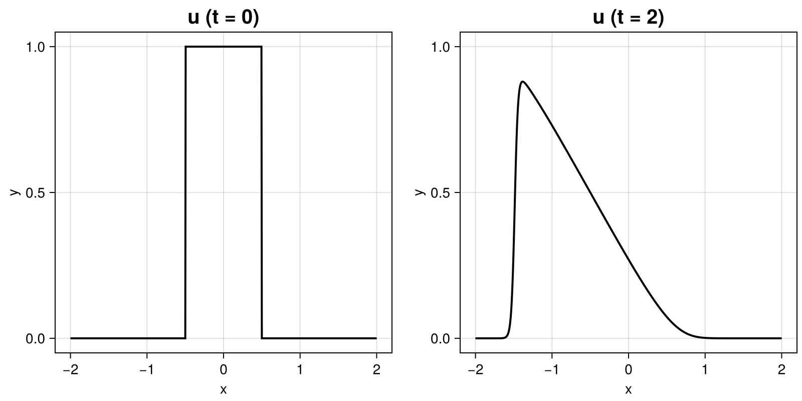
The initial condition and the final solution for the default parameters looks like this:
module Example103_BurgersEquation

using ExtendableFEM
using ExtendableGrids
using DifferentialEquations

# nonlinear kernel, i.e. f(u)
function f!(result, input, qpinfo)
	result[1] = input[1]^2 / 2
end

# initial condition
function uinit!(result, qpinfo)
	result[1] = abs(qpinfo.x[1]) < 0.5 ? 1 : 0
end

# everything is wrapped in a main function
function main(;
	ν = 0.01,
	h = 0.005,
	T = 2,
	order = 2,
	τ = 0.01,
	Plotter = nothing,
	use_diffeq = true,
	solver = Rosenbrock23(autodiff = false),
	kwargs...)

	# load mesh and exact solution
	xgrid = simplexgrid(-2:h:2)

	# generate empty PDEDescription for three unknowns (h, u)
	PD = ProblemDescription("Burger's Equation")
	u = Unknown("u"; name = "u")
	assign_unknown!(PD, u)
	assign_operator!(PD, NonlinearOperator(f!, [grad(u)], [id(u)]; bonus_quadorder = 2))
	assign_operator!(PD, BilinearOperator([grad(u)]; store = true, factor = ν))
	assign_operator!(PD, CombineDofs(u, u, [1], [num_nodes(xgrid)], [1.0]; kwargs...))

	# prepare solution vector and initial data
	FES = FESpace{H1Pk{1, 1, order}}(xgrid)
	sol = FEVector(FES; tags = PD.unknowns)
	interpolate!(sol[u], uinit!)

	# init plotter and plot u0
	plt = plot([id(u), id(u)], sol; Plotter = Plotter, title_add = " (t = 0)")

	# generate mass matrix
	M = FEMatrix(FES)
	assemble!(M, BilinearOperator([id(1)]; lump = 2))

	if (use_diffeq)
		# generate DifferentialEquations.ODEProblem
		prob = ExtendableFEM.generate_ODEProblem(PD, FES, (0.0, T); init = sol, mass_matrix = M)

		# solve ODE problem
		de_sol = DifferentialEquations.solve(prob, solver, abstol = 1e-6, reltol = 1e-3, dt = τ, dtmin = 1e-6, adaptive = true)
		@info "#tsteps = $(length(de_sol))"

		# extract final solution
		sol.entries .= de_sol[end]
	else
		# add backward Euler time derivative
		assign_operator!(PD, BilinearOperator(M, [u]; factor = 1 / τ, kwargs...))
		assign_operator!(PD, LinearOperator(M, [u], [u]; factor = 1 / τ, kwargs...))

		# generate solver configuration
		SC = SolverConfiguration(PD, FES; init = sol, maxiterations = 1, kwargs...)

		# iterate tspan
		t = 0
		for it ∈ 1:Int(floor(T / τ))
			t += τ
			ExtendableFEM.solve(PD, FES, SC; time = t)
		end
	end

	# plot final state
	plot!(plt, [id(u)], sol; keep = 1, title_add = " (t = $T)")

	return sol, plt
end

end
This page was generated using Literate.jl.