225 : Obstacle Problem
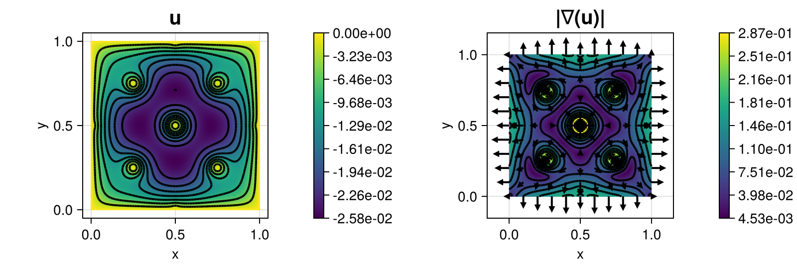
This example computes the solution $u$ of the nonlinear obstacle problem that seeks the minimiser of the energy functional
\[\begin{aligned} E(u) = \frac{1}{2} \int_\Omega \lvert \nabla u \rvert^2 dx - \int_\Omega f u dx \end{aligned}\]
with some right-hand side $f$ within the set of admissible functions that lie above an obstacle $\chi$
\[\begin{aligned} \mathcal{K} := \lbrace u \in H^1_0(\Omega) : u \geq \chi \rbrace. \end{aligned}\]
The obstacle constraint is realised via a penalty term
\[\begin{aligned} \frac{1}{\epsilon} \| \min(0, u - \chi) \|^2_{L^2} \end{aligned}\]
that is added to the energy above and is automatically differentiated for a Newton scheme. The computed solution for the default parameters looks like this:
module Example225_ObstacleProblem

using ExtendableFEM
using ExtendableGrids

# define obstacle and penalty kernel
const χ! = (result, x) -> (result[1] = (cos(4 * x[1] * π) * cos(4 * x[2] * π) - 1) / 20)
function obstacle_penalty_kernel!(result, input, qpinfo)
	χ!(result, qpinfo.x) # eval obstacle
	result[1] = min(0, input[1] - result[1])
	return nothing
end

function main(; Plotter = nothing, ϵ = 1e-4, nrefs = 6, order = 1, kwargs...)

	# choose initial mesh
	xgrid = uniform_refine(grid_unitsquare(Triangle2D), nrefs)

	# problem description
	PD = ProblemDescription()
	u = Unknown("u"; name = "potential")
	assign_unknown!(PD, u)
	assign_operator!(PD, NonlinearOperator(obstacle_penalty_kernel!, [id(u)]; factor = 1 / ϵ, kwargs...))
	assign_operator!(PD, BilinearOperator([grad(u)]; kwargs...))
	assign_operator!(PD, LinearOperator([id(u)]; factor = -1, kwargs...))
	assign_operator!(PD, HomogeneousBoundaryData(u; regions = 1:4, kwargs...))

	# create finite element space
	FES = FESpace{H1Pk{1, 2, order}}(xgrid)

	# solve
	sol = solve(PD, FES; kwargs...)

	# plot
	plt = plot([id(u), grad(u)], sol; Plotter = Plotter, ncols = 3)

	return sol, plt
end

end # module
This page was generated using Literate.jl.