206 : CoupledSubGridProblems
This example demonstrates how to solve a coupled problem where two variables only live on a sub-domain and are coupled through an interface condition. Consider the unit square domain cut in half through on of its diagonals. On each subdomain a solutiong $u_j$ of the two-dimensional Poisson problem
\[\begin{aligned} -\Delta u & = f \quad \text{in } \Omega \end{aligned}\]
with inhomogeneous boundary conditions on the former boundaries of the full square is searched. Along the common boundary between the two subdomains a new interface region is assigned (appended to BFaceNodes) and an interface condition is assembled that couples the two solutions $u_1$ and $u_2$ to each other. In this toy example, this interface conditions penalizes the jump between the two solutions on each side of the diagonal. Oberserve, that if the penalization factor $\tau$ is large, the two solutions are almost equal along the interface.
The computed solution(s) looks like this:
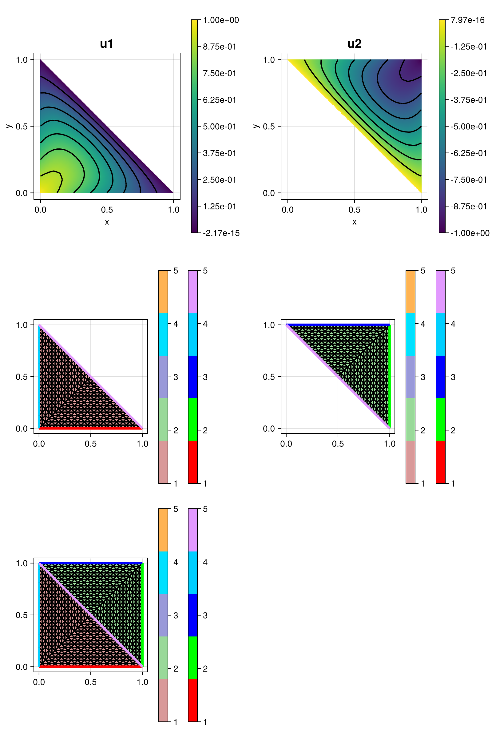
Each column of the plot shows the solution, the subgrid it lives on. The last row shows the full grid.
module Example206_CoupledSubGridProblems

using ExtendableFEM
using ExtendableGrids
using Test #


function boundary_conditions!(result, qpinfo)
    result[1] = 1 - qpinfo.x[1] - qpinfo.x[2] # used for both subsolutions
end

function interface_condition!(result, u, qpinfo)
    result[1] = u[1] - u[2]
    result[2] = -result[1]
end

function interface_condition_LM!(result, u, qpinfo)
    result[1] = (u[1] - u[2])
end


function main(; μ = [1.0,1.0], f = [10,-10], τ = 1, use_LM = true, nref = 4, order = 2, Plotter = nothing, kwargs...)

	# Finite element type
	FEType = H1Pk{1, 2, order}
    FETypeLM = H1Pk{1, 1, order}

	# generate mesh
	xgrid = grid_unitsquare(Triangle2D)

    # define regions
    xgrid[CellRegions] = Int32[1,2,2,1]

    # add an interface between region 1 and 2
    # (one can use the BFace storages for that)
    xgrid[BFaceNodes] = Int32[xgrid[BFaceNodes] [2 5; 5 4]]
    append!(xgrid[BFaceRegions], [5,5])
    xgrid[FaceRegions][xgrid[BFaceFaces][end-1:end]] .= 5
    xgrid[BFaceGeometries] = VectorOfConstants{ElementGeometries, Int}(Edge1D, 6)

    # refine
    xgrid = uniform_refine(xgrid, nref)

    # define an FESpace just on region 1 and one just on region 2
    FES1 = FESpace{FEType}(xgrid; regions = [1])
    FES2 = FESpace{FEType}(xgrid; regions = [2])
    if use_LM
        FES3 = FESpace{FETypeLM, ON_FACES}(xgrid; regions = [5])
        @show FES3.xgrid FES3.dofgrid
    end

    # define variables
    u1 = Unknown("u1"; name = "potential in region 1")
    u2 = Unknown("u2"; name = "potential in region 2")
    p = Unknown("p"; name = "LM for interface condition")

    # problem description
	PD = ProblemDescription()
	assign_unknown!(PD, u1)
	assign_unknown!(PD, u2)
	assign_operator!(PD, BilinearOperator([grad(u1)]; regions = [1], factor = μ[1], kwargs...))
	assign_operator!(PD, BilinearOperator([grad(u2)]; regions = [2], factor = μ[2], kwargs...))
    assign_operator!(PD, LinearOperator([id(u1)]; regions = [1], factor = f[1]))
    assign_operator!(PD, LinearOperator([id(u2)]; regions = [2], factor = f[2]))
    if use_LM
        assign_unknown!(PD, p)
        assign_operator!(PD, BilinearOperator(interface_condition_LM!, [id(p)], [id(u1), id(u2)]; regions = [5], transposed_copy = 1, entities = ON_FACES, kwargs...))
    else
	    assign_operator!(PD, BilinearOperator(interface_condition!, [id(u1), id(u2)]; regions = [5], factor = τ, entities = ON_FACES, kwargs...))
    end
	assign_operator!(PD, InterpolateBoundaryData(u1, boundary_conditions!; regions = 1:4))
	assign_operator!(PD, InterpolateBoundaryData(u2, boundary_conditions!; regions = 1:4))

    sol = solve(PD, use_LM ? [FES1, FES2, FES3] : [FES1, FES2])

    plt = plot([id(u1), id(u2), dofgrid(u1), dofgrid(u2), grid(u1)], sol; Plotter = Plotter)

	return sol, plt
end


end #module
This page was generated using Literate.jl.