203 : Poisson-Problem DG
This example computes the solution $u$ of the two-dimensional Poisson problem
\[\begin{aligned} -\Delta u & = f \quad \text{in } \Omega \end{aligned}\]
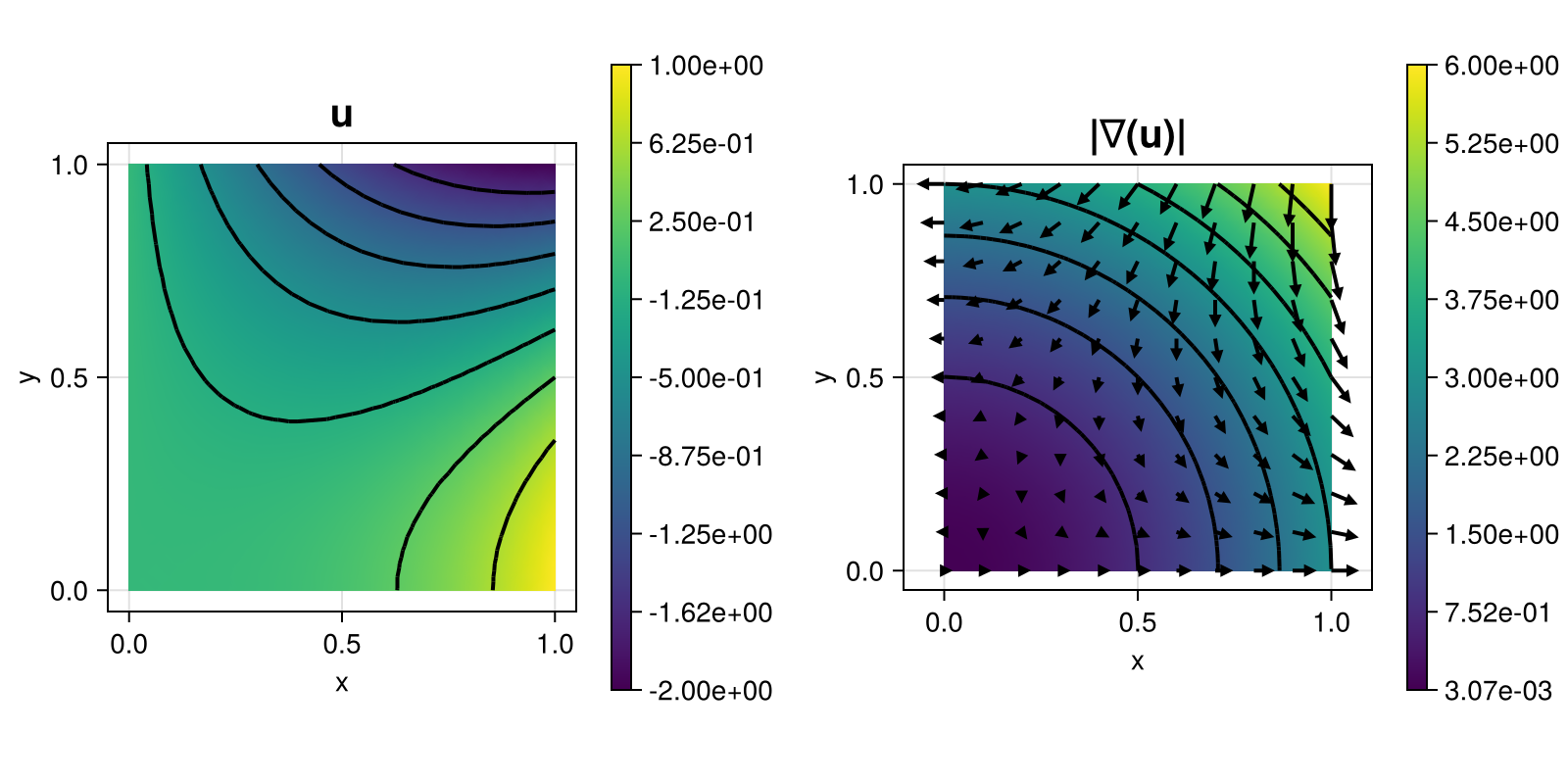
with right-hand side $f$ and inhomogeneous Dirichlet boundary conditions chosen such that $u(x,y) = x^3 - 3xy^2$. This time the problem is solved on a given grid via the discontinuous Galerkin method.
The computed solution looks like this:
module Example203_PoissonProblemDG

using ExtendableFEM
using ExtendableGrids
using LinearAlgebra
using Symbolics

# exact data for problem by Symbolics
function prepare_data(; μ = 1)

	@variables x y

	# exact solution
	u = x^3 - 3 * x * y^2
	∇u = Symbolics.gradient(u, [x, y])

	# right-hand side
	Δu = Symbolics.gradient(∇u[1], [x]) + Symbolics.gradient(∇u[2], [y])
	f = -μ * Δu[1]

	# build functions
	u_eval = build_function(u, x, y, expression = Val{false})
	∇u_eval = build_function(∇u, x, y, expression = Val{false})
	f_eval = build_function(f, x, y, expression = Val{false})
	return f_eval, u_eval, ∇u_eval[2]
end

function main(; dg = true, μ = 1.0, τ = 10.0, nrefs = 4, order = 2, bonus_quadorder = 2, Plotter = nothing, kwargs...)

	# prepare problem data
	f_eval, u_eval, ∇u_eval = prepare_data(; μ = μ)
	rhs!(result, qpinfo) = (result[1] = f_eval(qpinfo.x[1], qpinfo.x[2]))
	exact_u!(result, qpinfo) = (result[1] = u_eval(qpinfo.x[1], qpinfo.x[2]))
	exact_∇u!(result, qpinfo) = (∇u_eval(result, qpinfo.x[1], qpinfo.x[2]))

	# problem description
	PD = ProblemDescription("Poisson problem")
	u = Unknown("u"; name = "potential")
	assign_unknown!(PD, u)
	assign_operator!(PD, BilinearOperator([grad(u)]; factor = μ, kwargs...))
	assign_operator!(PD, LinearOperator(rhs!, [id(u)]; bonus_quadorder = bonus_quadorder, kwargs...))
	assign_operator!(PD, InterpolateBoundaryData(u, exact_u!; bonus_quadorder = bonus_quadorder, regions = 1:4))

	# discretize
	xgrid = uniform_refine(grid_unitsquare(Triangle2D), nrefs)
	FES = FESpace{order == 0 ? L2P0{1} : H1Pk{1, 2, order}}(xgrid; broken = dg)

	# add DG terms
	assign_operator!(PD, BilinearOperatorDG(dg_kernel, [jump(id(u))], [average(grad(u))]; entities = ON_FACES, factor = -μ, transposed_copy = 1, kwargs...))
	assign_operator!(PD, LinearOperatorDG(dg_kernel_bnd(exact_u!), [average(grad(u))]; entities = ON_BFACES, factor = -μ, bonus_quadorder = bonus_quadorder, kwargs...))
	assign_operator!(PD, BilinearOperatorDG(dg_kernel2, [jump(id(u))]; entities = ON_FACES, factor = μ*τ, kwargs...))
	assign_operator!(PD, LinearOperatorDG(dg_kernel2_bnd(exact_u!), [id(u)]; entities = ON_BFACES, regions = 1:4, factor = μ*τ, bonus_quadorder = bonus_quadorder, kwargs...))

	# solve
	sol = solve(PD, FES; kwargs...)

	# prepare error calculation
	function exact_error!(result, u, qpinfo)
		exact_u!(result, qpinfo)
		exact_∇u!(view(result, 2:3), qpinfo)
		result .-= u
		result .= result .^ 2
	end
	function dgjumps!(result, u, qpinfo)
		result .= u[1]^2/qpinfo.volume
	end
	ErrorIntegratorExact = ItemIntegrator(exact_error!, [id(u), grad(u)]; quadorder = 2 * (order+1), params = [μ], kwargs...)
	DGJumpsIntegrator = ItemIntegratorDG(dgjumps!, [jump(id(u))]; entities = ON_IFACES, kwargs...)

	# calculate error
	error = evaluate(ErrorIntegratorExact, sol)
	dgjumps = sqrt(sum(evaluate(DGJumpsIntegrator, sol)))
	L2error = sqrt(sum(view(error, 1, :)))
	H1error = sqrt(sum(view(error, 2, :)) + sum(view(error, 3, :)))
	@info "L2 error = $L2error"
	@info "H1 error = $H1error"
	@info "dgjumps = $dgjumps"

	# plot
	plt = plot([id(u), grad(u)], sol; Plotter = Plotter)

	return L2error, plt
end

function dg_kernel(result, input, qpinfo)
	result[1] = dot(input, qpinfo.normal)
end
function dg_kernel_bnd(uDb! = nothing)
	function closure(result, qpinfo)
		uDb!(result, qpinfo)
		result[1:2] = result[1] .* qpinfo.normal
	end
end
function dg_kernel2(result, input, qpinfo)
	result .= input / qpinfo.volume
end
function dg_kernel2_bnd(uDb! = nothing)
	function closure(result, qpinfo)
		uDb!(result, qpinfo)
		result /= qpinfo.volume
	end
end

end # module
This page was generated using Literate.jl.