226 : Thermoforming
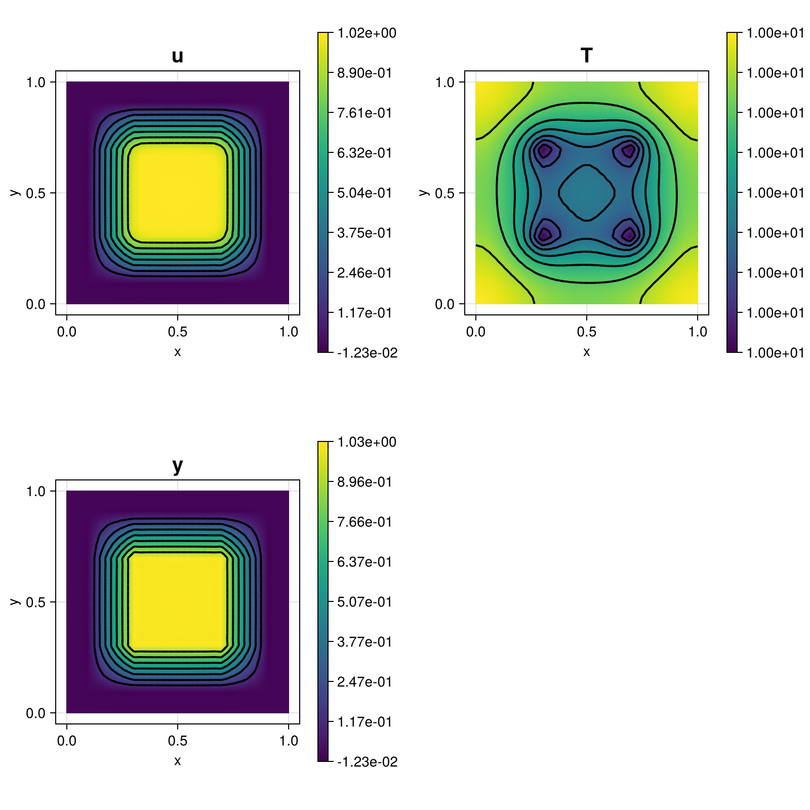
This implements the thermoforming example taken from https://arxiv.org/abs/1802.03564 Section 6.4. The computed solution for the default parameters looks like this:
module Example226_Thermoforming

using ExtendableFEM
using ExtendableGrids
using SparseArrays
using LinearAlgebra

function w(r)
	if 0.1 ≤ r ≤ 0.3
		return 5.0 * r - 0.5
	elseif 0.3 < r < 0.7
		return 1.0
	elseif 0.7 <= r <= 0.9
		return 4.5 - 5.0 * r
	else
		return 0.0
	end
end

# initial mould
function Φ0(x)
	return w(x[1]) * w(x[2])
end


function g(r,κ,s)
	if r <= 0.0
		return κ
	elseif r <= 0.25 * s
		return κ - 8.0 * κ * r^2 / (3.0 * s^2)
	elseif r <= 0.75 * s
		return 7.0 / 6.0 * κ - 4.0 / 3.0 * κ * r / s
	elseif r <= s
		return 8.0 / 3.0 * (s - r)^2 / s^2
	else
		return 0.0
	end
end


# The smooth bump function in [0,1]
bump(x) = (0.0 <= x <= 1.0) ? exp(-0.25 / (x - x^2)) : 0.0

# Bump in [0,1]^2
bumpInUnitSquare(x) = begin
	r = sqrt((x[1] - 0.5)^2 + (x[2] - 0.5)^2)
	return bump(0.5 + r)
end


# nonlinear kernel
function nonlinear_kernel!(result, input, qpinfo )
	# results and input contain 7 variables (u,∇u,T,∇T,y)
	u  = view(input, 1)
	∇u = view(input, 2:3)
	T  = view(input, 4)
	∇T = view(input, 5:6)
	y  = view(input, 7)

	α = qpinfo.params[1]
	k = qpinfo.params[2]
	f = qpinfo.params[3]
	β = qpinfo.params[4]
	κ = qpinfo.params[5]
	s = qpinfo.params[6]

	result[1]   = α * max(0, u[1] - y[1]) - f                                             # pattern: 1 7
	result[2:3] = ∇u                                                                      # pattern: 2 / 3
	result[4]   = k*T[1] - g(y[1]-u[1],κ,s)                                               # pattern: 1 4 7
	result[5:6] = ∇T                                                                      # pattern: 5 / 6
	result[7]   = y[1] - Φ0(qpinfo.x) - β * bumpInUnitSquare( qpinfo.x ) * T[1]           # pattern: 4 7
end

# custom sparsity pattern for the jacobians of the nonlinear_kernel (Symbolcs cannot handle conditional jumps)
# note: jacobians are defined row-wise
rows = [1, 1, 2, 3, 4, 4, 4, 5, 6, 7, 7]
cols = [1 ,7, 2, 3, 1, 4, 7, 5, 6, 4, 7]
vals = ones(Bool, length(cols))
sparsity_pattern = sparse(rows,cols,vals)

function main(;
	κ = 10,
	s = 1,
	α = 1e8,
	k = 1,
	β = 5.25e-3,
	f = 100,
	N = 32,
	order = 1,
	Plotter = nothing,
	kwargs...)

	# choose mesh,
	h = 1/(N+1)
	xgrid = simplexgrid(0:h:1,0:h:1)

	# problem description
	PD = ProblemDescription()
	u = Unknown("u"; name = "membrane position")
	y = Unknown("y"; name = "mould")
	T = Unknown("T"; name = "temperature")
	assign_unknown!(PD, u)
	assign_unknown!(PD, y)
	assign_unknown!(PD, T)
	assign_operator!(PD, NonlinearOperator(nonlinear_kernel!, [id(u), grad(u), id(T), grad(T), id(y)]; bonus_quadorder=2, params=[α,k,f,β,κ,s], sparse_jacobians_pattern=sparsity_pattern, kwargs...))
	assign_operator!(PD, HomogeneousBoundaryData(u; regions = 1:4, kwargs...))
	assign_operator!(PD, HomogeneousBoundaryData(y; regions = 1:4, kwargs...))

	# create finite element space
	FES = FESpace{H1Pk{1, 2, order}}(xgrid)
	FESs = [FES, FES, FES]
	sol = FEVector(FESs; tags = [u,y,T])

	# initial guess for Newton
	interpolate!(sol[u], (result,qpinfo) -> ( result[1] = 0.9*Φ0(qpinfo.x) ) )
	interpolate!(sol[T], (result,qpinfo) -> ( result[1] = 0.2 ) )
	interpolate!(sol[y], (result,qpinfo) -> ( result[1] = 10.0 ) )

	# solve
	sol = solve(PD, FESs; init = sol, maxiterations=420, target_residual=1e-8, kwargs...)

	# plot
	plt = plot([id(u),id(T),id(y)], sol; Plotter = Plotter)

	return sol, plt
end

end # module
This page was generated using Literate.jl.