265 : Flow + Transport
This example solve the Stokes problem in an Omega-shaped pipe and then uses the velocity in a transport equation for a species with a certain inlet concentration. Altogether, we are looking for a velocity $\mathbf{u}$, a pressure $\mathbf{p}$ and a stationary species concentration $\mathbf{c}$ such that
\[\begin{aligned} - \mu \Delta \mathbf{u} + \nabla p & = 0\\ \mathrm{div}(\mathbf{u}) & = 0\\ \mathbf{c}_t - \kappa \Delta \mathbf{c} + \mathbf{u} \cdot \nabla \mathbf{c} & = 0 \end{aligned}\]
with some viscosity parameter and diffusion parameter $\kappa$.
The diffusion coefficient for the species is chosen (almost) zero such that the isolines of the concentration should stay parallel from inlet to outlet. For the discretisation of the convection term in the transport equation three possibilities can be chosen:
- Classical Bernardi–Raugel stationary finite element discretisations $\mathbf{u}_h \cdot \nabla \mathbf{c}_h$ [set FVtransport = false, reconstruct = false]
- As in 1. but with divergence-free reconstruction operator in convection term $\Pi_\text{reconst} \mathbf{u}_h \cdot \nabla \mathbf{c}_h$ [set FVtransport = false, reconstruct = true]
- Time-dependent upwind finite volume discretisation for $\kappa = 0$ based on normal fluxes along the faces [set FVtransport = true]
Observe that the divergence-free postprocessing helps a lot for mass conservation, but is still not perfect. The finite volume upwind discretisation ensures mass conservation.
Note, that the transport equation is very convection-dominated and no stabilisation in the finite element discretisations was used here (but instead a nonzero $\kappa$). Also note, that only the finite volume discretisation perfectly obeys the maximum principle for the concentration but the isolines do no stay parallel until the outlet is reached, possibly due to articifial diffusion.
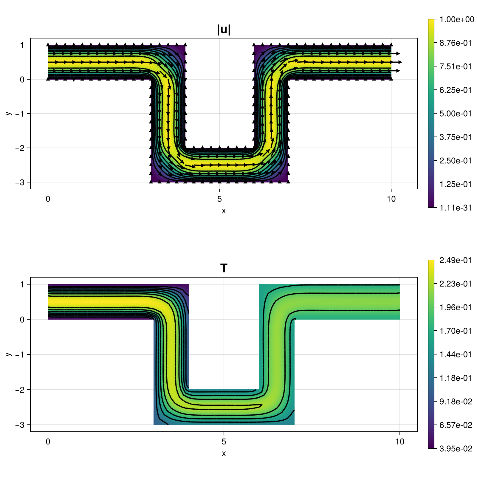
The computed solution for the default parameters looks like this:
module Example265_FlowTransport

using ExtendableFEM
using ExtendableGrids
using SimplexGridFactory
using Triangulate

# boundary data
function u_inlet!(result, qpinfo)
    x = qpinfo.x
    result[1] = 4*x[2]*(1-x[2])
    result[2] = 0
end
function c_inlet!(result, qpinfo)
    result[1] = (1-qpinfo.x[2])*qpinfo.x[2]
end

function kernel_stokes_standard!(result, u_ops, qpinfo)
    ∇u, p = view(u_ops,1:4), view(u_ops, 5)
    μ = qpinfo.params[1]
    result[1] = μ*∇u[1] - p[1]
    result[2] = μ*∇u[2]
    result[3] = μ*∇u[3]
    result[4] = μ*∇u[4] - p[1]
    result[5] = -(∇u[1] + ∇u[4])
end

function kernel_convection!(result, ∇T, u, qpinfo)
    result[1] = ∇T[1]*u[1] + ∇T[2]*u[2]
end

function kernel_inlet!(result, input, qpinfo)
    c_inlet!(result, qpinfo)
    result[1] *= -input[1]
end


# everything is wrapped in a main function
function main(; nrefs = 4, Plotter = nothing, reconstruct = true, FVtransport = true, μ = 1, kwargs...)

    # load mesh and refine
    xgrid = uniform_refine(simplexgrid(Triangulate;
    points = [0 0; 3 0; 3 -3; 7 -3; 7 0; 10 0; 10 1; 6 1; 6 -2; 4 -2; 4 1; 0 1]',
    bfaces = [1 2; 2 3; 3 4; 4 5; 5 6; 6 7; 7 8; 8 9; 9 10; 10 11; 11 12; 12 1]',
    bfaceregions = [1; 1; 1; 1; 1; 2; 3; 3; 3; 3; 3; 4],
    regionpoints = [0.5 0.5;]',
    regionnumbers = [1],
    regionvolumes = [1.0]), nrefs)

    # define unknowns
    u = Unknown("u"; name = "velocity", dim = 2)
    p = Unknown("p"; name = "pressure", dim = 1)
    T = Unknown("T"; name = "temperature", dim = 1)

    id_u = reconstruct ? apply(u, Reconstruct{HDIVBDM1{2}, Identity}) : id(u)

    # define first sub-problem: Stokes equations to solve for velocity u
    PD = ProblemDescription("Stokes problem")
    assign_unknown!(PD, u)
    assign_unknown!(PD, p)
    assign_operator!(PD, BilinearOperator(kernel_stokes_standard!, [grad(u), id(p)]; params = [μ], kwargs...))
    assign_operator!(PD, InterpolateBoundaryData(u, u_inlet!; regions = 4, kwargs...))
    assign_operator!(PD, HomogeneousBoundaryData(u; regions = [1,3], kwargs...))

    # add transport equation of species
    PDT = ProblemDescription("transport problem")
    assign_unknown!(PDT, T)
    if FVtransport ## FVM discretisation of transport equation (pure upwind convection)
        τ = 1e3
        assign_operator!(PDT, CallbackOperator(assemble_fv_operator!(), [u]; kwargs...))
        assign_operator!(PDT, BilinearOperator([id(T)]; store = true, factor = 1/τ, kwargs...))
        assign_operator!(PDT, LinearOperator([id(T)], [id(T)]; factor = 1/τ, kwargs...))
    else ## FEM discretisation of transport equation (with small diffusion term)
        assign_operator!(PDT, BilinearOperator([grad(T)]; factor = 1e-6, kwargs...))
        assign_operator!(PDT, BilinearOperator(kernel_convection!, [id(T)], [grad(T)], [id_u]; kwargs...))
        assign_operator!(PDT, InterpolateBoundaryData(T, c_inlet!; regions = [4], kwargs...))
    end

    # generate FESpaces and a solution vector for all 3 unknowns
    FETypes = [H1BR{2}, L2P0{1}, FVtransport ? L2P0{1} : H1P1{1}]
    FES = [FESpace{FETypes[j]}(xgrid) for j = 1 : 3]
    sol = FEVector(FES; tags = [u,p,T])

    # solve the two problems separately
    sol = solve(PD; init = sol, kwargs...)
    sol = solve(PDT; init = sol, maxiterations = 20, target_residual = 1e-12, constant_matrix = true, kwargs...)

    # print minimal and maximal concentration to check max principle (shoule be in [0,1])
    println("\n[min(c),max(c)] = [$(minimum(view(sol[T]))),$(maximum(view(sol[T])))]")

    # plot
    plt = plot([id(u), id(T)], sol; Plotter = Plotter, ncols = 1, spacing = 0.25, width = 800, height = 800)

    return sol, plt
end

# pure convection finite volume operator for transport
function assemble_fv_operator!()

    BndFluxIntegrator = ItemIntegrator(kernel_inflow!, [normalflux(1)]; entities = ON_BFACES)
    FluxIntegrator = ItemIntegrator([normalflux(1)]; entities = ON_FACES)
    fluxes::Matrix{Float64} = zeros(Float64,1,0)

    function closure(A, b, args; assemble_matrix = true, assemble_rhs = true, kwargs...)

    # prepare grid and stash
    xgrid = args[1].FES.xgrid
    nfaces = size(xgrid[FaceCells],2)
    if size(fluxes,2) < nfaces
        fluxes = zeros(Float64, 1, nfaces)
    end

    # right-hand side = boundary inflow fluxes if velocity points inward
    if assemble_rhs
        fill!(fluxes, 0)
        evaluate!(fluxes, BndFluxIntegrator, [args[1]])
        facecells = xgrid[FaceCells]
        bface2face = xgrid[BFaceFaces]
        for bface in 1 : lastindex(bface2face)
            b[facecells[1, bface2face[bface]]] -= fluxes[bface]
        end
    end

    # assemble upwind finite volume fluxes over cell faces into matrix
    if assemble_matrix
        # integrate normalfux of velocity
        fill!(fluxes, 0)
        evaluate!(fluxes, FluxIntegrator, [args[1]])

        cellfaces = xgrid[CellFaces]
        cellfacesigns = xgrid[CellFaceSigns]
        for cell = 1 : num_cells(xgrid)
            nfaces4cell = num_targets(cellfaces, cell)
            for cf = 1 : nfaces4cell
                face = cellfaces[cf,cell]
                other_cell = facecells[1,face]
                if other_cell == cell
                    other_cell = facecells[2,face]
                end
                flux = fluxes[face] * cellfacesigns[cf,cell]
                if (other_cell > 0)
                    flux *= 1 // 2 # because it will be accumulated on two cells
                end
                if flux > 0 # flow from cell to other_cell or out of domain
                    _addnz(A,cell,cell,flux,1)
                    if other_cell > 0
                        _addnz(A,other_cell,cell,-flux,1)
                        # otherwise flow goes out of domain
                    end
                else # flow from other_cell into cell or into domain
                    _addnz(A,cell,cell,1e-16,1) # add zero to keep pattern for LU
                    if other_cell > 0 # flow comes from neighbour cell
                        _addnz(A,other_cell,other_cell,-flux,1)
                        _addnz(A,cell,other_cell,flux,1)
                    end
                    # otherwise flow comes from outside into domain, handled in rhs side loop above
                end
            end
        end
    end
    return nothing
    end
end


function kernel_inflow!(result, input, qpinfo)
    if input[1] < 0 # if velocity points into domain
        c_inlet!(result, qpinfo)
        result[1] *= input[1]
    else
        result[1] = 0
    end
end

end # module
This page was generated using Literate.jl.