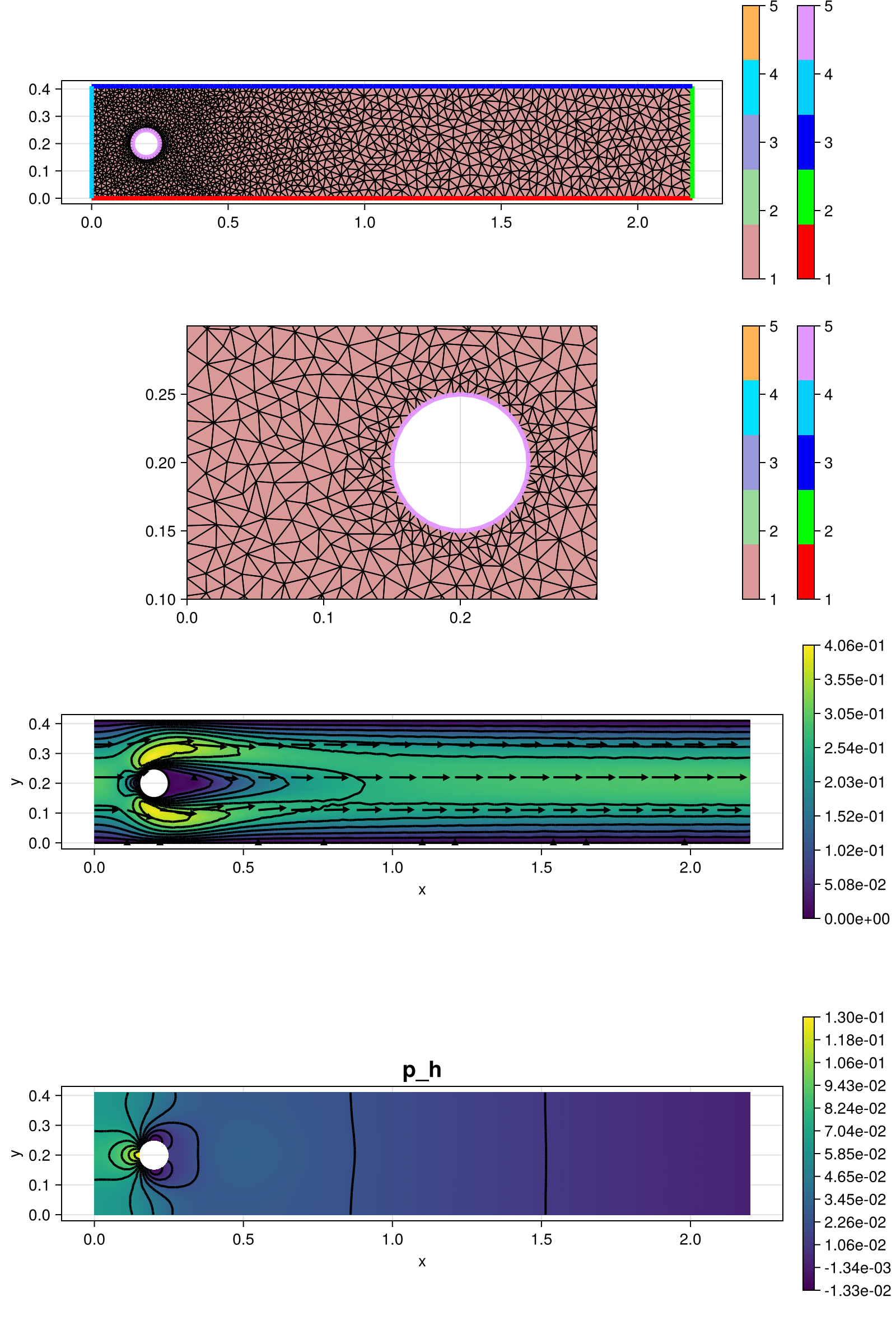
245 : Flow around a cylinder
This example solves the DFG Navier-Stokes benchmark problem
\[\begin{aligned} - \mu \Delta \mathbf{u} + (\mathbf{u} \cdot \nabla) \mathbf{u} + \nabla p & = 0\\ \mathrm{div}(\mathbf{u}) & = 0 \end{aligned}\]
on a rectangular 2D domain with a circular obstacle, see here for details.
This script demonstrates the employment of external grid generators and the computation of drag and lift coefficients.
Note: This example needs the additional packages Triangulate and SimplexGridFactory to generate the mesh.
module Example245_NSEFlowAroundCylinder

using ExtendableFEM
using Triangulate
using SimplexGridFactory
using ExtendableGrids
using GridVisualize
using LinearAlgebra

# inlet data for Karman vortex street example
# as in DFG benchmark 2D-1 (Re = 20, laminar)
const umax = 0.3
const umean = 2 // 3 * umax
const L, W, H = 0.1, 2.2, 0.41
function inflow!(result, qpinfo)
	x = qpinfo.x
	result[1] = 4 * umax * x[2] * (H - x[2]) / (H * H)
	result[2] = 0.0
end

# hand constructed identity matrix for kernel to avoid allocations
const II = [1 0; 0 1]


# Example of a kernel using tensor_view() function to allow for an operator
# based style of writing the semilinear form.
# For comparison we also provide the kernel_nonlinear_flat! function below
# that uses a component-wise style of writing the semilinear form.

#
# the scalar product ``(\nabla v, \mu \nabla u - p)`` will be evaluated
# so in general `a = b` corresponds to ``(a,b)``.

# Note that the order of vector entries between the kernel and the call to
# NonlinearOperator have to match.
function kernel_nonlinear!(result, u_ops, qpinfo)
Shape values of vectorial u are starting at index 1 view as 1-tensor(vector) of length dim=2 in 2D
    u = tensor_view(u_ops, 1, TDVector(2))
    v = tensor_view(result, 1, TDVector(2))
gradients of vectorial u are starting at index 3 view as 2-tensor of size 2x2 in 2D
    ∇u = tensor_view(u_ops, 3, TDMatrix(2))
    ∇v = tensor_view(result, 3, TDMatrix(2))
values of scalar p are starting at index 7 view as 0-tensor (single value)
    p = tensor_view(u_ops, 7, TDScalar())
    q = tensor_view(result, 7, TDScalar())
get viscosity at current quadrature point
μ = qpinfo.params[1]Note that all operators should be element-wise to avoid allocations (v,u⋅∇u) = (v,∇u^T⋅u)
tmul!(v,∇u,u)(∇v,μ∇u-p)
∇v .= μ .* ∇u .- p[1] .* II(q,-∇⋅u)
    q[1] = -dot(∇u, II)
    return nothing
end


# everything is wrapped in a main function
function main(; Plotter = nothing, μ = 1e-3, maxvol = 1e-3, reconstruct = true, kwargs...)

	# load grid (see function below)
	xgrid = make_grid(W, H; n = Int(ceil(sqrt(1 / maxvol))), maxvol = maxvol)

	# problem description
	PD = ProblemDescription()
	u = Unknown("u"; name = "velocity")
	p = Unknown("p"; name = "pressure")
	id_u = reconstruct ? apply(u, Reconstruct{HDIVRT1{2}, Identity}) : id(u)

	assign_unknown!(PD, u)
	assign_unknown!(PD, p)
	assign_operator!(PD, NonlinearOperator(kernel_nonlinear!, [id_u, grad(u), id(p)]; params = [μ], kwargs...))
	assign_operator!(PD, InterpolateBoundaryData(u, inflow!; regions = 4))
	assign_operator!(PD, HomogeneousBoundaryData(u; regions = [1, 3, 5]))

	# P2-bubble + reconstruction operator
	FETypes = [H1P2B{2, 2}, H1P1{1}]

	# generate FESpaces and Solution vector
	FES = [FESpace{FETypes[1]}(xgrid), FESpace{FETypes[2]}(xgrid; broken = true)]

	# solve
	sol = solve(PD, FES; maxiterations = 50, target_residual = 1e-10)

	# postprocess : compute drag/lift (see function below)
	draglift = get_draglift(sol, μ)
	pdiff = get_pressure_difference(sol)
	println("[drag, lift] = $draglift")
	println("p difference = $pdiff")

	# plots via GridVisualize
	plt = GridVisualizer(; Plotter = Plotter, layout = (4, 1), clear = true, size = (800, 1200))
	gridplot!(plt[1, 1], xgrid, linewidth = 1)
	gridplot!(plt[2, 1], xgrid, linewidth = 1, xlimits = [0, 0.3], ylimits = [0.1, 0.3])
	scalarplot!(plt[3, 1], xgrid, nodevalues(sol[u]; abs = true)[1, :])
	vectorplot!(plt[3, 1], xgrid, eval_func_bary(PointEvaluator([id(u)], sol)), spacing = (0.2, 0.05), vscale = 0.5, clear = false)
	scalarplot!(plt[4, 1], xgrid, view(nodevalues(sol[p]), 1, :), levels = 11, title = "p_h")

	return [draglift[1], draglift[2], pdiff[1]], plt
end

function get_pressure_difference(sol::FEVector)
	xgrid = sol[2].FES.xgrid
	PE = PointEvaluator([id(2)], sol)
	p_left = zeros(Float64, 1)
	x1 = [0.15, 0.2]
	p_right = zeros(Float64, 1)
	x2 = [0.25, 0.2]
	evaluate!(p_left, PE, x1)
	evaluate!(p_right, PE, x2)
	@show p_left, p_right
	return p_left - p_right
end

function get_draglift(sol::FEVector, μ)

	# this function is interpolated for drag/lift test function creation
	function DL_testfunction(component)
		function closure(result, qpinfo)
			x = qpinfo.x
			fill!(result, 0)
			if sqrt((x[1] - 0.2)^2 + (x[2] - 0.2)^2) <= 0.06
				result[component] = 1
			end
		end
	end

	# drag lift calcuation by testfunctions
	function draglift_kernel(result, input, qpinfo)
		# input = [ u, grad(u), p , v , grad(v)]
		#         [1:2,  3:6,   7 ,8:9,  10:13 ]
		result[1] = μ * (input[3] * input[10] + input[4] * input[11] + input[5] * input[12] + input[6] * input[13])
		result[1] += (input[1] * input[3] + input[2] * input[4]) * input[8]
		result[1] += (input[1] * input[5] + input[2] * input[6]) * input[9]
		result[1] -= input[7] * (input[10] + input[13])
		result[1] *= -(2 / (umean^2 * L))
		return nothing
	end
	DLIntegrator = ItemIntegrator(draglift_kernel, [id(1), grad(1), id(2), id(3), grad(3)]; quadorder = 4)

	# test for drag
	TestFunction = FEVector(sol[1].FES; name = "drag/lift testfunction")
	interpolate!(TestFunction[1], ON_BFACES, DL_testfunction(1))
	drag = sum(evaluate(DLIntegrator, [sol[1], sol[2], TestFunction[1]]))

	# test for lift
	interpolate!(TestFunction[1], ON_BFACES, DL_testfunction(2))
	lift = sum(evaluate(DLIntegrator, [sol[1], sol[2], TestFunction[1]]))

	return [drag, lift]
end

# grid generator script using SimplexGridBuilder/Triangulate
function make_grid(W, H; n = 20, maxvol = 0.1)
	builder = SimplexGridBuilder(Generator = Triangulate)
	function circlehole!(builder, center, radius; n = 20)
		points = [point!(builder, center[1] + radius * sin(t), center[2] + radius * cos(t)) for t in range(0, 2π, length = n)]
		for i ∈ 1:n-1
			facet!(builder, points[i], points[i+1])
		end
		facet!(builder, points[end], points[1])
		holepoint!(builder, center)
	end
	p1 = point!(builder, 0, 0)
	p2 = point!(builder, W, 0)
	p3 = point!(builder, W, H)
	p4 = point!(builder, 0, H)

	# heuristic refinement around cylinder
	refine_radius = 0.25
	maxrefinefactor = 1 // 20
	function unsuitable(x1, y1, x2, y2, x3, y3, area)
		if area > maxvol * min(max(4 * maxrefinefactor, abs((x1 + x2 + x3) / 3 - 0.2)), 1 / maxrefinefactor)
			return true
		end
		dist = sqrt(((x1 + x2 + x3) / 3 - 0.2)^2 + ((y1 + y2 + y3) / 3 - 0.2)^2) - 0.05
		myarea = dist < refine_radius ? maxvol * max(maxrefinefactor, 1 - (refine_radius - dist) / refine_radius) : maxvol
		if area > myarea
			return true
		else
			return false
		end
	end

	facetregion!(builder, 1)
	facet!(builder, p1, p2)
	facetregion!(builder, 2)
	facet!(builder, p2, p3)
	facetregion!(builder, 3)
	facet!(builder, p3, p4)
	facetregion!(builder, 4)
	facet!(builder, p4, p1)
	facetregion!(builder, 5)
	circlehole!(builder, (0.2, 0.2), 0.05, n = n)

	simplexgrid(builder, maxvolume = 16 * maxvol, unsuitable = unsuitable)
end

end
This page was generated using Literate.jl.