211 : Poisson L-shape Local Equilibrated Fluxes
This example computes a local equilibration error estimator for the $H^1$ error of some $H^1$-conforming approximation $u_h$ to the solution $u$ of some Poisson problem $-\Delta u = f$ on an L-shaped domain, i.e.
\[\eta^2(\sigma_h) := \| \sigma_h - \nabla u_h \|^2_{L^2(T)}\]
where $\sigma_h$ discretisates the exact $\sigma$ in the dual mixed problem
\[\sigma - \nabla u = 0 \quad \text{and} \quad \mathrm{div}(\sigma) + f = 0\]
by some local equilibration strategy, see reference below for details.
This examples demonstrates the use of low-level structures to assemble individual problems and a strategy to solve several small problems in parallel by use of non-overlapping node patch groups.
''A posteriori error estimates for efficiency and error control in numerical simulations'' Lecture Notes by M. Vohralik >Link<
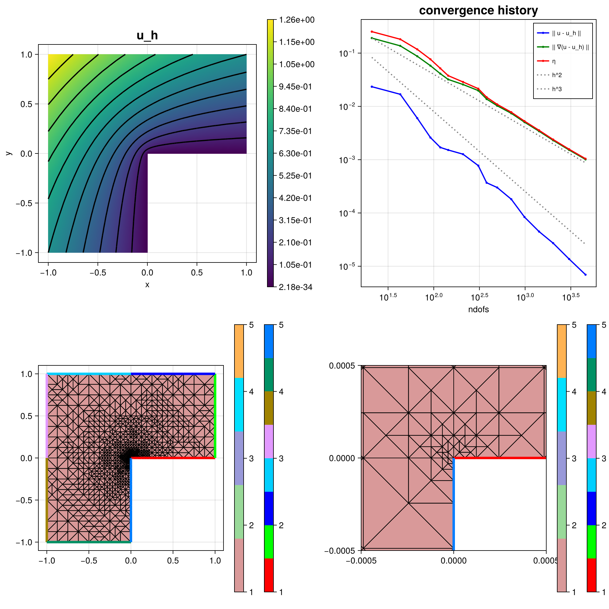
The resulting mesh and error convergence history for the default parameters looks like:
module Example211_LshapeAdaptiveEQPoissonProblem

using ExtendableFEM
using ExtendableFEMBase
using ExtendableGrids
using ExtendableSparse
using GridVisualize

# exact solution u for the Poisson problem
function u!(result, qpinfo)
	x = qpinfo.x
	r2 = x[1]^2 + x[2]^2
	φ = atan(x[2], x[1])
	if φ < 0
		φ += 2 * pi
	end
	result[1] = r2^(1 / 3) * sin(2 * φ / 3)
end

# gradient of exact solution
function ∇u!(result, qpinfo)
	x = qpinfo.x
	φ = atan(x[2], x[1])
	r2 = x[1]^2 + x[2]^2
	if φ < 0
		φ += 2 * pi
	end
	∂r = 2 / 3 * r2^(-1 / 6) * sin(2 * φ / 3)
	∂φ = 2 / 3 * r2^(-1 / 6) * cos(2 * φ / 3)
	result[1] = cos(φ) * ∂r - sin(φ) * ∂φ
	result[2] = sin(φ) * ∂r + cos(φ) * ∂φ
end

# kernel for exact error calculation
function exact_error!(result, u, qpinfo)
	u!(result, qpinfo)
	∇u!(view(result, 2:3), qpinfo)
	result .-= u
	result .= result .^ 2
end

# kernel for equilibration error estimator
function eqestimator_kernel!(result, input, qpinfo)
	σ_h, divσ_h, ∇u_h = view(input, 1:2), input[3], view(input, 4:5)
	result[1] = norm(σ_h .- ∇u_h)^2 + divσ_h^2
	return nothing
end

# unknowns for primal and dual problem
u = Unknown("u"; name = "u")
σ = Unknown("σ"; name = "equilibrated fluxes / dual stress")

# everything is wrapped in a main function
function main(; maxdofs = 4000, μ = 1, order = 2, nlevels = 16, θ = 0.5, Plotter = nothing, kwargs...)

	# initial grid
	xgrid = grid_lshape(Triangle2D)

	# choose some finite elements for primal and dual problem (= for equilibrated fluxes)
	FEType = H1Pk{1,2,order}
	FETypeDual = HDIVRTk{2, order}

	# setup Poisson problem
	PD = ProblemDescription("Poisson problem")
	assign_unknown!(PD, u)
	assign_operator!(PD, BilinearOperator([grad(u)]; factor = μ, kwargs...))
	assign_operator!(PD, InterpolateBoundaryData(u, u!; regions = 2:7, bonus_quadorder = 4, kwargs...))
	assign_operator!(PD, HomogeneousBoundaryData(u; regions = [1, 8]))

	# define error estimator : || σ_h - ∇u_h ||^2 + || div σ_h ||^2
	EQIntegrator = ItemIntegrator(eqestimator_kernel!, [id(σ), div(σ), grad(u)]; resultdim = 1, quadorder = 2 * order)

	# setup exact error evaluations
	ErrorIntegrator = ItemIntegrator(exact_error!, [id(u), grad(u)]; quadorder = 2 * order, kwargs...)

	# refinement loop (only uniform for now)
	NDofs = zeros(Int, 0)
	NDofsDual = zeros(Int, 0)
	ResultsL2 = zeros(Float64, 0)
	ResultsH1 = zeros(Float64, 0)
	Resultsη = zeros(Float64, 0)
	sol = nothing
	level = 0
	while (true)
		level += 1

		# create a solution vector and solve the problem
		FES = FESpace{FEType}(xgrid)
		sol = solve(PD, FES)
		push!(NDofs, length(view(sol[u])))
		println("\n  SOLVE LEVEL $level")
		println("    ndofs = $(NDofs[end])")

		# evaluate eqilibration error estimator and append it to sol vector (for plotting etc.)
		local_equilibration_estimator!(sol, FETypeDual)
		η4cell = evaluate(EQIntegrator, sol)
		push!(Resultsη, sqrt(sum(view(η4cell, 1, :))))

		# calculate L2 error, H1 error, estimator, dual L2 error and write to results
		push!(NDofsDual, length(view(sol[σ])))
		error = evaluate(ErrorIntegrator, sol)
		push!(ResultsL2, sqrt(sum(view(error, 1, :))))
		push!(ResultsH1, sqrt(sum(view(error, 2, :)) + sum(view(error, 3, :))))
		println("  ESTIMATE")
		println("    ndofsDual = $(NDofsDual[end])")
		println("    estim H1 error = $(Resultsη[end])")
		println("    exact H1 error = $(ResultsH1[end])")
		println("    exact L2 error = $(ResultsL2[end])")

		if NDofs[end] >= maxdofs
			break
		end

		# mesh refinement
		if θ >= 1 ## uniform mesh refinement
			xgrid = uniform_refine(xgrid)
		else ## adaptive mesh refinement
			facemarker = bulk_mark(xgrid, view(η4cell, :), θ; indicator_AT = ON_CELLS)
			xgrid = RGB_refine(xgrid, facemarker)
		end
	end

	# plot
	plt = GridVisualizer(; Plotter = Plotter, layout = (2, 2), clear = true, resolution = (1000, 1000))
	scalarplot!(plt[1, 1], id(u), sol; levels = 11, title = "u_h")
	plot_convergencehistory!(plt[1, 2], NDofs, [ResultsL2 ResultsH1 Resultsη]; add_h_powers = [order, order + 1], X_to_h = X -> order * X .^ (-1 / 2), ylabels = ["|| u - u_h ||", "|| ∇(u - u_h) ||", "η"])
	gridplot!(plt[2, 1], xgrid; linewidth = 1)
	gridplot!(plt[2, 2], xgrid; linewidth = 1, xlimits = [-0.0005, 0.0005], ylimits = [-0.0005, 0.0005])

	# print/plot convergence history
	print_convergencehistory(NDofs, [ResultsL2 ResultsH1 Resultsη]; X_to_h = X -> X .^ (-1 / 2), ylabels = ["|| u - u_h ||", "|| ∇(u - u_h) ||", "η"])

	return sol, plt
end

# this function computes the local equilibrated fluxes
# by solving local problems on (disjunct groups of) node patches
function local_equilibration_estimator!(sol, FETypeDual)
	# needed grid stuff
	xgrid = sol[u].FES.xgrid
	xCellNodes::Array{Int32, 2} = xgrid[CellNodes]
	xCellVolumes::Array{Float64, 1} = xgrid[CellVolumes]
	xNodeCells::Adjacency{Int32} = atranspose(xCellNodes)
	nnodes::Int = num_sources(xNodeCells)

	# get node patch groups that can be solved in parallel
	group4node = xgrid[NodePatchGroups]

	# init equilibration space (and Lagrange multiplier space)
	FESDual = FESpace{FETypeDual}(xgrid)
	xItemDofs::Union{VariableTargetAdjacency{Int32}, SerialVariableTargetAdjacency{Int32}, Array{Int32, 2}} = FESDual[CellDofs]
	xItemDofs_uh::Union{VariableTargetAdjacency{Int32}, SerialVariableTargetAdjacency{Int32}, Array{Int32, 2}} = sol[u].FES[CellDofs]

	# append block in solution vector for equilibrated fluxes
	append!(sol, FESDual; tag = σ)

	# partition of unity and their gradients = P1 basis functions
	POUFES = FESpace{H1P1{1}}(xgrid)
	POUqf = QuadratureRule{Float64, Triangle2D}(0)

	# quadrature formulas
	qf = QuadratureRule{Float64, Triangle2D}(2 * get_polynomialorder(FETypeDual, Triangle2D))
	weights::Array{Float64, 1} = qf.w

	# some constants
	offset::Int = sol[u].offset
	div_penalty::Float64 = 1e5      # divergence constraint is realized by penalisation
	bnd_penalty::Float64 = 1e60     # penalty for non-involved dofs of a group
	maxdofs::Int = max_num_targets_per_source(xItemDofs)
	maxdofs_uh::Int = max_num_targets_per_source(xItemDofs_uh)

	# redistribute groups for more equilibrated thread load (first groups are larger)
	maxgroups = maximum(group4node)
	groups = Array{Int, 1}(1:maxgroups)
	for j::Int ∈ 1:floor(maxgroups / 2)
		a = groups[j]
		groups[j] = groups[2*j]
		groups[2*j] = a
	end
	X = Array{Array{Float64, 1}, 1}(undef, maxgroups)

	function solve_patchgroup!(group)
		# temporary variables
		graduh = zeros(Float64, 2)
		coeffs_uh = zeros(Float64, maxdofs_uh)
		Alocal = zeros(Float64, maxdofs, maxdofs)
		blocal = zeros(Float64, maxdofs)

		# init system
		A = ExtendableSparseMatrix{Float64, Int64}(FESDual.ndofs, FESDual.ndofs)
		b = zeros(Float64, FESDual.ndofs)

		# init FEBasiEvaluators
		FEE_∇φ = FEEvaluator(POUFES, Gradient, POUqf)
		FEE_xref = FEEvaluator(POUFES, Identity, qf)
		FEE_∇u = FEEvaluator(sol[u].FES, Gradient, qf)
		FEE_div = FEEvaluator(FESDual, Divergence, qf)
		FEE_id = FEEvaluator(FESDual, Identity, qf)
		idvals = FEE_id.cvals
		divvals = FEE_div.cvals
		xref_vals = FEE_xref.cvals
		∇φvals = FEE_∇φ.cvals

		# find dofs at boundary of current node patches
		# and in interior of cells outside of current node patch group
		is_noninvolveddof = zeros(Bool, FESDual.ndofs)
		outside_cell::Bool = false
		for cell ∈ 1:num_cells(xgrid)
			outside_cell = true
			for k ∈ 1:3
				if group4node[xCellNodes[k, cell]] == group
					outside_cell = false
					break
				end
			end
			if (outside_cell) # mark interior dofs of outside cell
				for j ∈ 1:maxdofs
					is_noninvolveddof[xItemDofs[j, cell]] = true
				end
			end
		end

		for node ∈ 1:nnodes
			if group4node[node] == group
				for c ∈ 1:num_targets(xNodeCells, node)
					cell = xNodeCells[c, node]

					# find local node number of global node z
					# and evaluate (constant) gradient of nodal basis function phi_z
					localnode = 1
					while xCellNodes[localnode, cell] != node
						localnode += 1
					end
					FEE_∇φ.citem[] = cell
					update_basis!(FEE_∇φ)

					# read coefficients for discrete flux
					for j ∈ 1:maxdofs_uh
						coeffs_uh[j] = sol.entries[offset + xItemDofs_uh[j, cell]]
					end

					# update other FE evaluators
					FEE_∇u.citem[] = cell
					FEE_div.citem[] = cell
					FEE_id.citem[] = cell
					update_basis!(FEE_∇u)
					update_basis!(FEE_div)
					update_basis!(FEE_id)

					# assembly on this cell
					for i in eachindex(weights)
						weight = weights[i] * xCellVolumes[cell]

						# evaluate grad(u_h) and nodal basis function at quadrature point
						fill!(graduh, 0)
						eval_febe!(graduh, FEE_∇u, coeffs_uh, i)

						# compute residual -f*phi_z + grad(u_h) * grad(phi_z) at quadrature point i ( f = 0 in this example !!! )
						temp2 = div_penalty * sqrt(xCellVolumes[cell]) * weight
						temp = temp2 * dot(graduh, view(∇φvals,:,localnode,1))
						for dof_i ∈ 1:maxdofs
							# right-hand side for best-approximation (grad(u_h)*phi)
							blocal[dof_i] += dot(graduh, view(idvals,:,dof_i, i)) * xref_vals[1, localnode, i] * weight
							# mass matrix Hdiv
							for dof_j ∈ dof_i:maxdofs
								Alocal[dof_i, dof_j] += dot(view(idvals,:,dof_i, i), view(idvals,:,dof_j, i)) * weight
							end
							# div-div matrix Hdiv * penalty (quick and dirty to avoid Lagrange multiplier)
							blocal[dof_i] += temp * divvals[1,dof_i,i]
							temp3 = temp2 * divvals[1,dof_i,i]
							for dof_j ∈ dof_i:maxdofs
								Alocal[dof_i, dof_j] += temp3 * divvals[1,dof_j,i]
							end
						end
					end

					# write into global A and b
					for dof_i ∈ 1:maxdofs
						dofi = xItemDofs[dof_i, cell]
						b[dofi] += blocal[dof_i]
						for dof_j ∈ 1:maxdofs
							dofj = xItemDofs[dof_j, cell]
							if dof_j < dof_i # use that Alocal is symmetric
								_addnz(A, dofi, dofj, Alocal[dof_j, dof_i], 1)
							else
								_addnz(A, dofi, dofj, Alocal[dof_i, dof_j], 1)
							end
						end
					end

					# reset local A and b
					fill!(Alocal, 0)
					fill!(blocal, 0)
				end
			end
		end

		# penalize dofs that are not involved
		for j ∈ 1:FESDual.ndofs
			if is_noninvolveddof[j]
				A[j, j] = bnd_penalty
				b[j] = 0
			end
		end

		# solve local problem
		return A \ b
	end

	# solve equilibration problems on vertex patches (in parallel)
	Threads.@threads for group in groups
		grouptime = @elapsed begin
			@info "  Starting equilibrating patch group $group on thread $(Threads.threadid())... "
			X[group] = solve_patchgroup!(group)
		end
		@info "Finished equilibration patch group $group on thread $(Threads.threadid()) in $(grouptime)s "
	end

	# write local solutions to global vector (sequentially)
	for group ∈ 1:maxgroups
		view(sol[σ]) .+= X[group]
	end
end

end
This page was generated using Literate.jl.