285 : Cahn-Hilliard Equations
This example studies the mixed form of the Cahn-Hilliard equations that seeks $(c,\mu)$ such that
\[\begin{aligned} c_t - \mathbf{div} (M \nabla \mu) & = 0\\ \mu - \partial f / \partial c + \lambda \nabla^2c & = 0. \end{aligned}\]
with $f(c) = 100c^2(1-c)^2$, constant parameters $M$ and $\lambda$ and (random) initial concentration as defined in the code below.
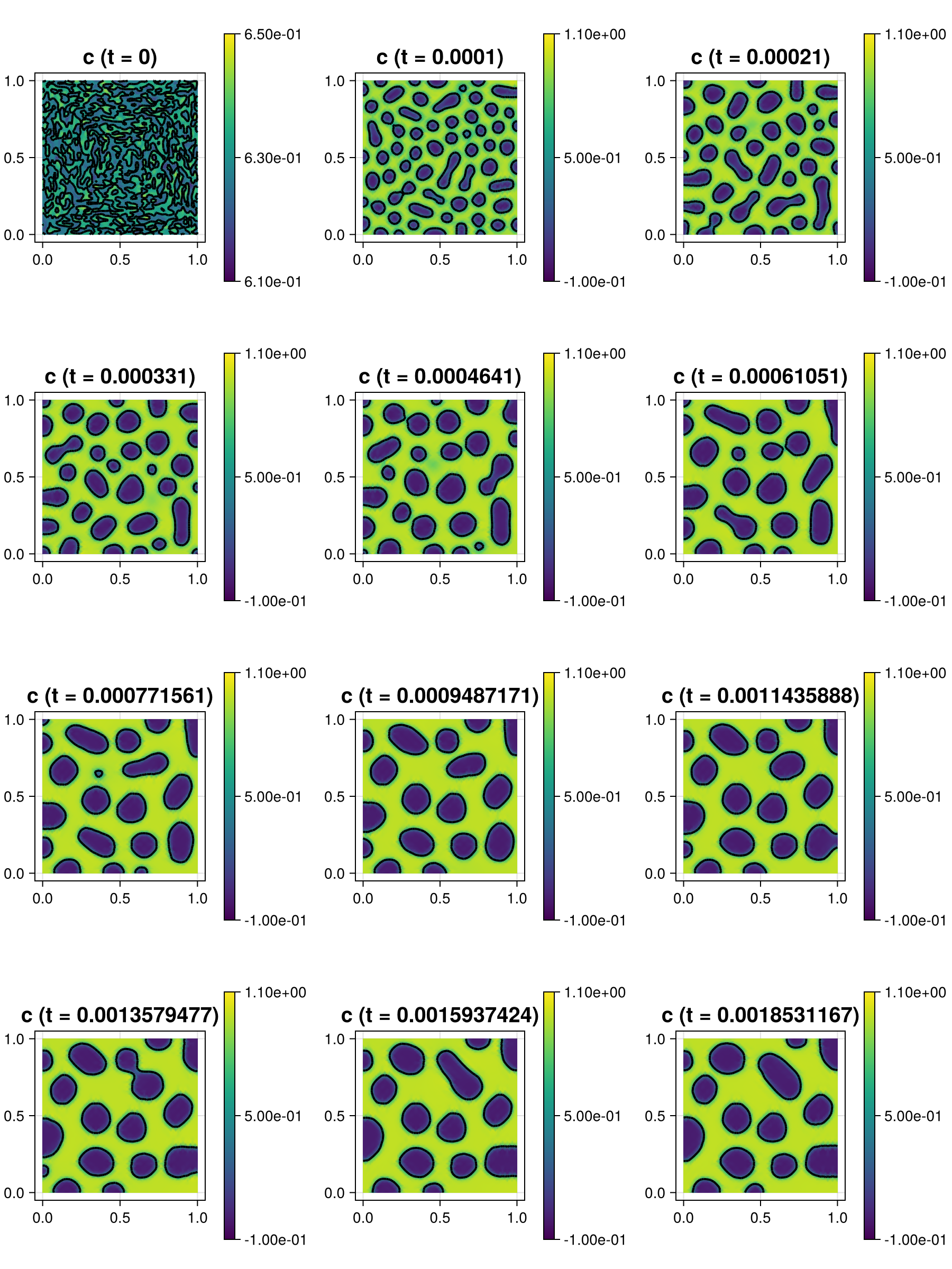
The computed solution at different timesteps for the default parameters and a randomized initial state look like this:
module Example285_CahnHilliard

using ExtendableFEM
using ExtendableGrids
using GridVisualize
using ForwardDiff
using Random
Random.seed!(135791113)

# parameters and initial condition
const f = (c) -> 100 * c^2 * (1 - c)^2
const dfdc = (c) -> ForwardDiff.derivative(f, c)

function c0!(result, qpinfo)
	result[1] = 0.63 + 0.02 * (0.5 - rand())
end

# everything is wrapped in a main function
function main(;
	order = 2,                              # finite element order for c and μ
	nref = 4,                               # refinement level
	M = 1.0,
	λ = 1e-2,
	iterations_until_next_plot = 20,
	τ = 5 / 1000000,                        # time step (for main evolution phase)
	τ_increase = 1.1,                      # increase factor for τ after each plot
	Plotter = nothing,                      # Plotter (e.g. PyPlot)
	kwargs...,
)

	# initial grid and final time
	xgrid = uniform_refine(grid_unitsquare(Triangle2D), nref)

	# define unknowns
	c = Unknown("c"; name = "concentration", dim = 1)
	μ = Unknown("μ"; name = "chemical potential", dim = 1)

	# define main level set problem
	PD = ProblemDescription("Cahn-Hilliard equation")
	assign_unknown!(PD, c)
	assign_unknown!(PD, μ)
	assign_operator!(PD, BilinearOperator([grad(c)], [grad(μ)]; factor = M, store = true))
	assign_operator!(PD, BilinearOperator([id(μ)]; store = true))
	assign_operator!(PD, BilinearOperator([grad(μ)], [grad(c)]; factor = -λ, store = true))

	# add nonlinear reaction part (= -df/dc times test function)
	function kernel_dfdc!(result, input, qpinfo)
		result[1] = -dfdc(input[1])
	end
	assign_operator!(PD, NonlinearOperator(kernel_dfdc!, [id(μ)], [id(c)]; bonus_quadorder = 1))

	# generate FESpace and solution vector and interpolate initial state
	FES = FESpace{H1Pk{1, 2, order}}(xgrid)
	sol = FEVector([FES, FES]; tags = PD.unknowns)
	interpolate!(sol[c], c0!)

	# init plot (if order > 1, solution is upscaled to finer grid for plotting)
	plt = GridVisualizer(; Plotter = Plotter, layout = (4, 3), clear = true, resolution = (900, 1200))
	if order > 1
		xgrid_upscale = uniform_refine(xgrid, order - 1)
		SolutionUpscaled = FEVector(FESpace{H1P1{1}}(xgrid_upscale))
		lazy_interpolate!(SolutionUpscaled[1], sol)
	else
		xgrid_upscale = xgrid
		SolutionUpscaled = sol
	end
	nodevals = nodevalues_view(SolutionUpscaled[1])
	scalarplot!(plt[1, 1], xgrid_upscale, nodevals[1]; limits = (0.61, 0.65), xlabel = "", ylabel = "", levels = 1, title = "c (t = 0)")

	# prepare backward Euler time derivative
	M = FEMatrix(FES)
	b = FEVector(FES)
	assemble!(M, BilinearOperator([id(1)]; factor = 1.0 / τ))
	assign_operator!(PD, BilinearOperator(M, [c]; kwargs...))
	assign_operator!(PD, LinearOperator(b, [c]; kwargs...))

	# generate solver configuration
	SC = SolverConfiguration(PD, [FES, FES]; init = sol, maxiterations = 50, target_residual = 1e-6, kwargs...)

	# advance in time, plot from time to time
	t = 0
	for j ∈ 1:11
		# do some timesteps until next plot
		for it ∈ 1:iterations_until_next_plot
			t += τ
			# update time derivative
			b.entries .= M.entries * view(sol[c])
			ExtendableFEM.solve(PD, [FES, FES], SC; time = t)
		end

		# enlarge time step a little bit
		τ *= τ_increase
		M.entries.cscmatrix.nzval ./= τ_increase

		# plot at current time
		if order > 1
			lazy_interpolate!(SolutionUpscaled[1], sol)
		end
		scalarplot!(plt[1+Int(floor((j) / 3)), 1+(j)%3], xgrid_upscale, nodevals[1]; xlabel = "", ylabel = "", limits = (-0.1, 1.1), levels = 1, title = "c (t = $(Float32(t)))")
	end

	return sol, plt
end

end
This page was generated using Literate.jl.