Example210_LshapeAdaptivePoissonProblem

(source code)

This example computes the standard-residual error estimator for the $H^1$ error $e = u - u_h$ of some $H^1$-conforming approximation $u_h$ to the solution $u$ of some Poisson problem $-\Delta u = f$ on an L-shaped domain, i.e.

\[\eta^2(u_h) := \sum_{T \in \mathcal{T}} \lvert T \rvert \| f + \Delta u_h \|^2_{L^2(T)} + \sum_{F \in \mathcal{F}} \lvert F \rvert \| [[\nabla u_h \cdot \mathbf{n}]] \|^2_{L^2(F)}\]

This example script showcases the evaluation of 2nd order derivatives like the Laplacian and adaptive mesh refinement.

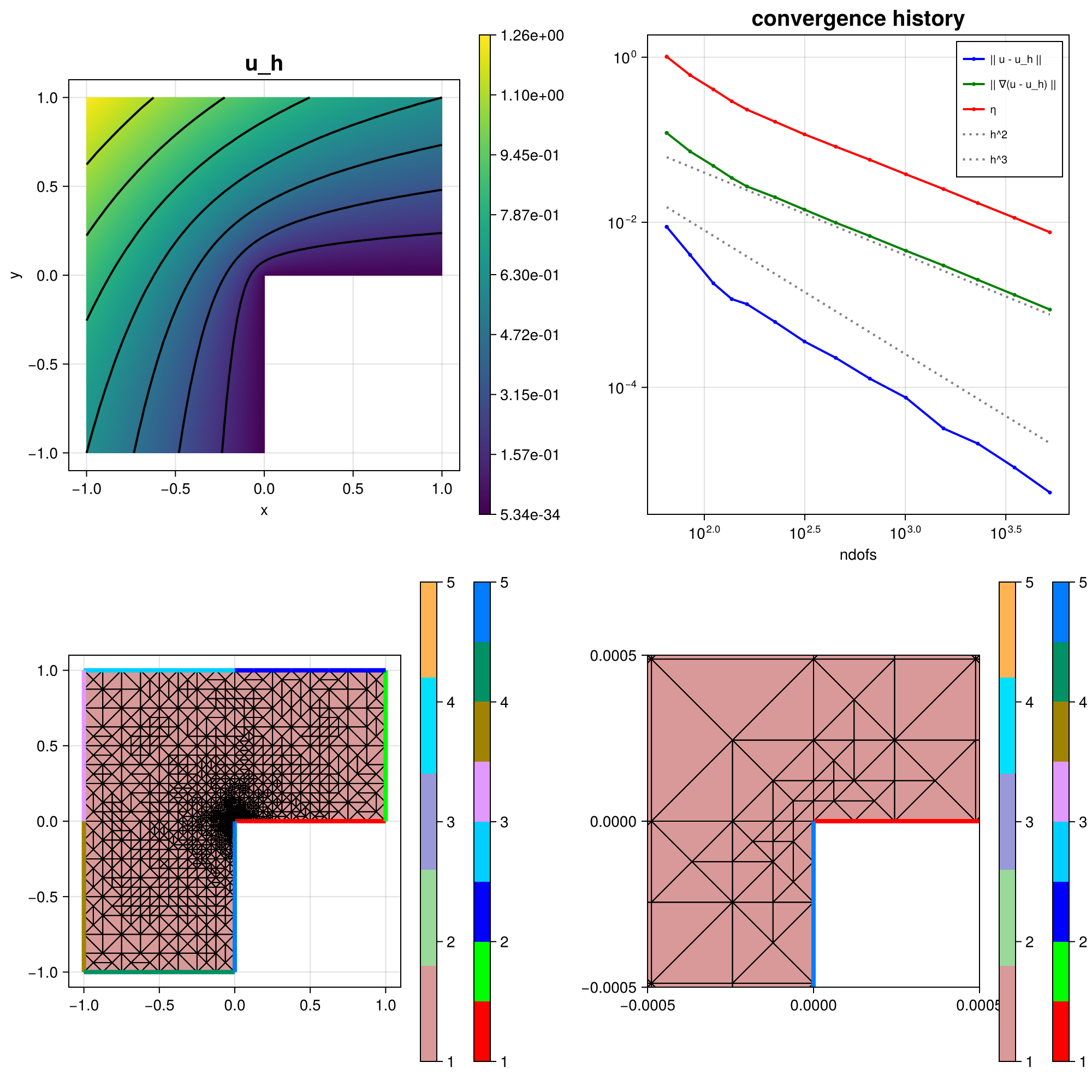
The resulting mesh and error convergence history for the default parameters looks like:

module Example210_LshapeAdaptivePoissonProblem

using ExtendableFEM
using GridVisualize
using ExtendableGrids
using LinearAlgebra

# exact solution u for the Poisson problem
function u!(result, qpinfo)
	x = qpinfo.x
	r2 = x[1]^2 + x[2]^2
	φ = atan(x[2], x[1])
	if φ < 0
		φ += 2 * pi
	end
	result[1] = r2^(1 / 3) * sin(2 * φ / 3)
end

# gradient of exact solution
function ∇u!(result, qpinfo)
	x = qpinfo.x
	φ = atan(x[2], x[1])
	r2 = x[1]^2 + x[2]^2
	if φ < 0
		φ += 2 * pi
	end
	∂r = 2 / 3 * r2^(-1 / 6) * sin(2 * φ / 3)
	∂φ = 2 / 3 * r2^(-1 / 6) * cos(2 * φ / 3)
	result[1] = cos(φ) * ∂r - sin(φ) * ∂φ
	result[2] = sin(φ) * ∂r + cos(φ) * ∂φ
end

# kernel for exact error calculation
function exact_error!(result, u, qpinfo)
	u!(result, qpinfo)
	∇u!(view(result, 2:3), qpinfo)
	result .-= u
	result .= result .^ 2
end

# kernel for face interpolation of normal jumps of gradient
function gradnormalflux!(result, ∇u, qpinfo)
	result[1] = dot(∇u, qpinfo.normal)
end

# kernel for face refinement indicator
function η_face!(result, gradjump, qpinfo)
	result .= qpinfo.volume * gradjump .^ 2
end

# kernel for cell refinement indicator
function η_cell!(result, Δu, qpinfo)
	result .= qpinfo.volume * Δu .^ 2
end

function main(; maxdofs = 4000, θ = 0.5, μ = 1.0, nrefs = 1, order = 2, Plotter = nothing, kwargs...)

	# problem description
	PD = ProblemDescription("Poisson problem")
	u = Unknown("u"; name = "u")
	assign_unknown!(PD, u)
	assign_operator!(PD, BilinearOperator([grad(u)]; factor = μ, kwargs...))
	assign_operator!(PD, InterpolateBoundaryData(u, u!; regions = 2:7, bonus_quadorder = 4, kwargs...))
	assign_operator!(PD, HomogeneousBoundaryData(u; regions = [1, 8]))

	# discretize
	xgrid = uniform_refine(grid_lshape(Triangle2D), nrefs)

	# define interpolators and item integrators for error estimation and calculation
	NormalJumpProjector = FaceInterpolator(gradnormalflux!, [jump(grad(u))]; resultdim = 1, order = order, only_interior = true, kwargs...)
	ErrorIntegratorFace = ItemIntegrator(η_face!, [id(1)]; quadorder = 2 * order, entities = ON_FACES, kwargs...)
	ErrorIntegratorCell = ItemIntegrator(η_cell!, [Δ(1)]; quadorder = 2 * (order - 2), entities = ON_CELLS, kwargs...)
	ErrorIntegratorExact = ItemIntegrator(exact_error!, [id(1), grad(1)]; quadorder = 2 * order, kwargs...)

	NDofs = zeros(Int, 0)
	ResultsL2 = zeros(Float64, 0)
	ResultsH1 = zeros(Float64, 0)
	Resultsη = zeros(Float64, 0)
	sol = nothing
	ndofs = 0
	level = 0
	while ndofs < maxdofs
		level += 1

		# SOLVE : create a solution vector and solve the problem
		println("------- LEVEL $level")
		if ndofs < 1000
			println(stdout, unicode_gridplot(xgrid))
		end
		@time begin
			# solve
			FES = FESpace{H1Pk{1, 2, order}}(xgrid)
			sol = ExtendableFEM.solve(PD, FES; u = [u], kwargs...)
			ndofs = length(sol[1])
			push!(NDofs, ndofs)
			println("\t ndof =  $ndofs")
			print("@time  solver =")
		end

		# ESTIMATE : calculate local error estimator contributions
		@time begin
			# calculate error estimator
			Jumps4Faces = evaluate!(NormalJumpProjector, sol)
			η_F = evaluate(ErrorIntegratorFace, Jumps4Faces)

			η_T = evaluate(ErrorIntegratorCell, sol)
			facecells = xgrid[FaceCells]
			for face ∈ 1:size(facecells, 2)
				η_F[face] += η_T[facecells[1, face]]
				if facecells[2, face] > 0
					η_F[face] += η_T[facecells[2, face]]
				end
			end

			# calculate total estimator
			push!(Resultsη, sqrt(sum(η_F)))
			print("@time  η eval =")
		end

		# calculate exact L2 error, H1 error
		@time begin
			error = evaluate(ErrorIntegratorExact, sol)
			push!(ResultsL2, sqrt(sum(view(error, 1, :))))
			push!(ResultsH1, sqrt(sum(view(error, 2, :)) + sum(view(error, 3, :))))
			print("@time  e eval =")
		end

		if ndofs >= maxdofs
			break
		end

		# MARK+REFINE : mesh refinement
		@time begin
			if θ >= 1 ## uniform mesh refinement
				xgrid = uniform_refine(xgrid)
			else ## adaptive mesh refinement
				# refine by red-green-blue refinement (incl. closuring)
				facemarker = bulk_mark(xgrid, view(η_F, :), θ; indicator_AT = ON_FACES)
				xgrid = RGB_refine(xgrid, facemarker)
			end
			print("@time  refine =")
		end
		println("\t    η =  $(Resultsη[level])\n\t    e =  $(ResultsH1[level])")
	end

	# plot
	plt = GridVisualizer(; Plotter = Plotter, layout = (2, 2), clear = true, size = (1000, 1000))
	scalarplot!(plt[1, 1], id(u), sol; levels = 7, title = "u_h")
	plot_convergencehistory!(plt[1, 2], NDofs, [ResultsL2 ResultsH1 Resultsη]; add_h_powers = [order, order + 1], X_to_h = X -> order * X .^ (-1 / 2), ylabels = ["|| u - u_h ||", "|| ∇(u - u_h) ||", "η"])
	gridplot!(plt[2, 1], xgrid; linewidth = 1)
	gridplot!(plt[2, 2], xgrid; linewidth = 1, xlimits = [-0.0005, 0.0005], ylimits = [-0.0005, 0.0005])

	# print convergence history
	print_convergencehistory(NDofs, [ResultsL2 ResultsH1 Resultsη]; X_to_h = X -> X .^ (-1 / 2), ylabels = ["|| u - u_h ||", "|| ∇(u - u_h) ||", "η"])

	return sol, plt
end

end # module

This page was generated using Literate.jl.

210 : Poisson L-shape Adaptive Mesh Refinement