275 : Optimal Control Stokes

(source code)

This example studies the optimal control problem for the Stokes operator with divergence-free velocity space $\mathbf{V}_0 \subset \mathbf{H}^1_0$, i.e., for given data $\mathbf{u}^d$ minimize the functional

\[\begin{aligned} \min_{(\mathbf{u},\mathbf{q}) \in \mathbf{V}_0 \times \mathbf{L}^2} \| \mathbf{u} - \mathbf{u}^d \|^2 + \frac{\alpha}{2} \| \mathbf{q} \|^2 \quad \text{s.t. } (\mu \nabla \mathbf{u}, \nabla \mathbf{v}) = (\mathbf{q}, \mathbf{v}) \quad \text{for all } \mathbf{v} \in \mathbf{V}_0 \end{aligned}\]

This results in the set of variational equations that seeks $(\mathbf{u}, \mathbf{z}, p , \lambda)$ such that

\[\begin{aligned} (\mu \nabla \mathbf{u}, \nabla \mathbf{v}) + (p, \mathrm{div} \mathbf{v}) & = - \alpha^{-1/2} (\mathbf{z}, \mathbf{v})\\ (q, \mathrm{div} \mathbf{u}) & = 0\\ (\mu \nabla \mathbf{z}, \nabla \mathbf{w}) + (λ, \mathrm{div} \mathbf{w}) & = \alpha^{-1/2} (\mathbf{u} - \mathbf{u}^d, \mathbf{w})\\ (φ, \mathrm{div} \mathbf{z}) & = 0. \end{aligned}\]

for all test functions $(\mathbf{v}, \mathbf{w}, q , \varphi)$.

Here, we study pressure-robustness with the given data

\[\mathbf{u}^d := \mathrm{curl} \left(x^4y^4(x-1)^4(y-1)^4\right) + \epsilon \nabla(\cos(x)\sin(y))\]

with a gradient field distortion that can be steered by $ϵ \geq 0$ which was an example in the reference below.

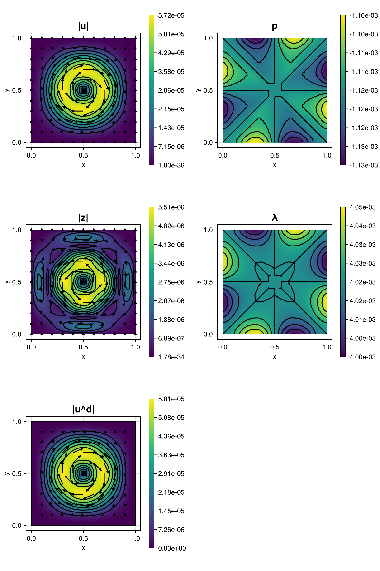
The computed solution for the default parameters looks like this:

module Example275_OptimalControlStokes

using ExtendableFEM
using ExtendableGrids
using Symbolics

function prepare_data!(; ϵ = 0)
	@variables x y

	# stream function ξ
	ξ = x^4*y^4*(x-1)^4*(y-1)^4
	∇ξ = Symbolics.gradient(ξ, [x,y])

    # irrotational perturbation (to study pressure-robustness)
    ϕ = cos(x)*sin(y)
	∇ϕ = Symbolics.gradient(ϕ, [x,y])

    # final data = curl ξ + ϵ ∇ϕ
	d = [-∇ξ[2], ∇ξ[1]] + ϵ * ∇ϕ
	d_eval = build_function(d, x, y, expression = Val{false})

    return d_eval[2]
end

# standard Stokes kernel
function kernel_stokes_standard!(result, u_ops, qpinfo)
    ∇u, p = view(u_ops,1:4), view(u_ops, 5)
    μ = qpinfo.params[1]
    result[1] = μ*∇u[1] + p[1]
    result[2] = μ*∇u[2]
    result[3] = μ*∇u[3]
    result[4] = μ*∇u[4] + p[1]
    result[5] = (∇u[1] + ∇u[4])
end

# everything is wrapped in a main function
function main(; nrefs = 4, Plotter = nothing, reconstruct = true, μ = 1, α = 1e-6, ϵ = 0, kwargs...)

    # prepare target data
    d_eval = prepare_data!(; ϵ = ϵ)
    data!(result, qpinfo) = (d_eval(result, qpinfo.x[1], qpinfo.x[2]);)

    # load mesh and refine
    xgrid = uniform_refine(grid_unitsquare(Triangle2D),nrefs)

    # define unknowns
    u = Unknown("u"; name = "velocity", dim = 2)
    z = Unknown("z"; name = "control", dim = 2)
    p = Unknown("p"; name = "pressure", dim = 1)
    λ = Unknown("λ"; name = "control pressure", dim = 1)

    # prepare reconstruction operator (if reconstruct = true)
    idR(u) = reconstruct ? apply(u, Reconstruct{HDIVBDM1{2}, Identity}) : id(u)

    # define optimal control problem
    PD = ProblemDescription("Stokes optimal control problem")
    assign_unknown!(PD, u)
    assign_unknown!(PD, z)
    assign_unknown!(PD, p)
    assign_unknown!(PD, λ)
    assign_operator!(PD, BilinearOperator(kernel_stokes_standard!, [grad(u), id(p)]; params = [μ], kwargs...))
    assign_operator!(PD, BilinearOperator(kernel_stokes_standard!, [grad(z), id(λ)]; params = [μ], kwargs...))
    assign_operator!(PD, BilinearOperator([idR(z)], [idR(u)]; factor = -1/sqrt(α), transposed_copy = -1, kwargs...))
    assign_operator!(PD, LinearOperator(data!, [idR(z)]; factor = -1/sqrt(α), bonus_quadorder = 5, kwargs...))
    assign_operator!(PD, HomogeneousBoundaryData(u; regions = 1:4, kwargs...))
    assign_operator!(PD, HomogeneousBoundaryData(z; regions = 1:4, kwargs...))

    # solve with Bernardi--Raugel method
    FETypes = [H1BR{2}, L2P0{1}]
    FES = [FESpace{FETypes[j]}(xgrid) for j = 1 : 2]
    sol = solve(PD, [FES[1],FES[1],FES[2],FES[2]]; kwargs...)

    # plot solution
    plt = plot([id(u), id(p), id(z), id(λ)], sol; add = 1, Plotter = Plotter)

    # plot target data
    I = FEVector(FES[1]; name = "u^d")
    interpolate!(I[1], data!)
    plot!(plt, [id(1)], I; keep = 1:4)

    return sol, plt
end

end

This page was generated using Literate.jl.