101 : L2-Bestapproximation 1D
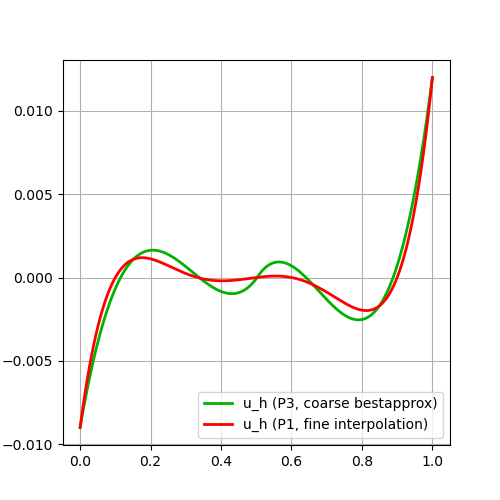
This example computes the L2-bestapproximation of some given scalar-valued function into the piecewise quadratic continuous polynomials. Afterwards the L2 error is computed and the solution is plotted.
module Example101_Bestapproximation1D

using GradientRobustMultiPhysics
using ExtendableGrids
using GridVisualize

# define some (vector-valued) function (to be L2-bestapproximated in this example)
function exact_function!(result,x)
    result[1] = (x[1]-1//2)*(x[1]-9//10)*(x[1]-1//3)*(x[1]-1//10)*(x[1]-0.6)
end
const u = DataFunction(exact_function!, [1,1]; name = "u", dependencies = "X", bonus_quadorder = 5)

# everything is wrapped in a main function
function main(; Plotter = nothing, verbosity = 0, order = 3, h = 0.5, h_fine = 1e-3)

    # set log level
    set_verbosity(verbosity)

    # generate coarse and fine mesh
    xgrid = simplexgrid(0:h:1)
    xgrid_fine = simplexgrid(0:h_fine:1)

    # setup a bestapproximation problem via a predefined prototype
    # and an L2ErrorEvaluator that can be used later to compute the L2 error
    Problem = L2BestapproximationProblem(u; bestapprox_boundary_regions = [1,2])
    L2ErrorEvaluator = L2ErrorIntegrator(u, Identity)

    # choose finite element type of desired order and generate a FESpace for the grid
    FEType = H1Pk{1,1,order}
    FES = FESpace{FEType}(xgrid)

    # generate a solution vector and solve the problem on the coarse grid
    Solution = FEVector(FES)
    solve!(Solution, Problem)

    # we want to compare our discrete solution with a finer P1 interpolation of u
    FES_fine = FESpace{H1P1{1}}(xgrid_fine)
    Interpolation = FEVector("Iu (fine)",FES_fine)
    interpolate!(Interpolation[1], u)

    # calculate the L2 errors
    L2error = sqrt(evaluate(L2ErrorEvaluator,Solution[1]))
    L2error_fine = (sqrt(evaluate(L2ErrorEvaluator,Interpolation[1])))
    println("\t|| u - u_h (P$order, coarse)|| = $L2error")
    println("\t|| u - u_h (P1, fine) ||= $L2error_fine")

    # since plots only use values at vertices, we upscale our (possibly higher order Solution)
    # by interpolating it also into a P1 function on the fine mesh
    SolutionUpscaled = FEVector("u_h (fine)",FES_fine)
    interpolate!(SolutionUpscaled[1], Solution[1])

    # evaluate/interpolate function at nodes and plot_trisurf
    p=GridVisualizer(Plotter=Plotter,layout=(1,1))
    scalarplot!(p[1,1],xgrid_fine, nodevalues_view(SolutionUpscaled[1])[1], color=(0,0.7,0), label = "u_h (P$order, coarse bestapprox)")
    scalarplot!(p[1,1],xgrid_fine, nodevalues_view(Interpolation[1])[1], clear = false, color = (1,0,0), label = "u_h (P1, fine interpolation)", legend = :rb)
end

end
This page was generated using Literate.jl.