250 : Level Set Method 2D
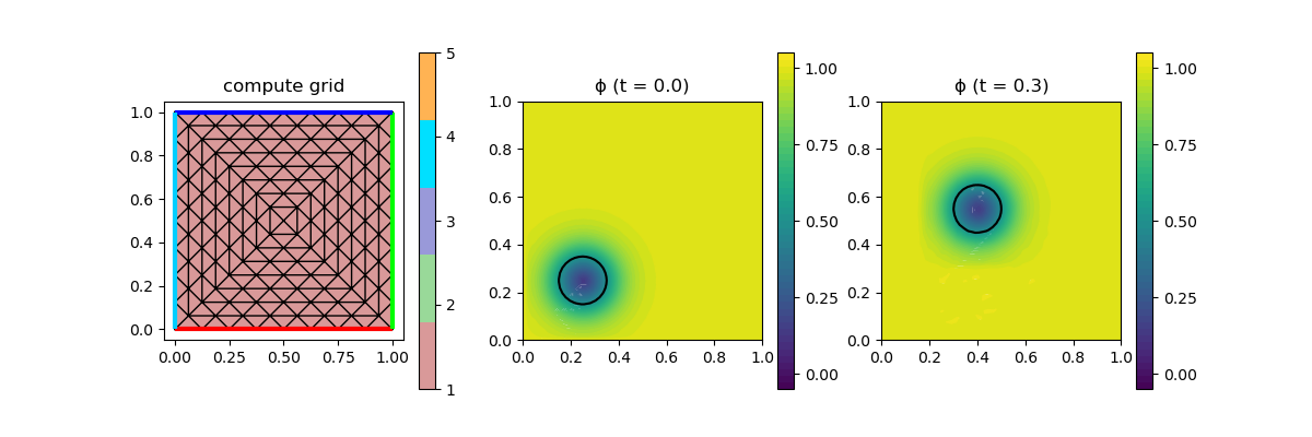
This example studies the level-set method of some level function $\mathbf{\phi}$ convected in time via the equation
\[\begin{aligned} \phi_t + \mathbf{u} \cdot \nabla \phi & = 0. \end{aligned}\]
Here this is tested with the (conservative) initial level set function $\phi(x) = 0.5 \tanh((\lvert x - (0.25,0.25) \rvert - 0.1)/(2ϵ) + 1)$ such that the level $\phi \equiv 0.5$ forms a circle which is then convected by the velocity $\mathbf{u} = (0.5,1)^T$. No reinitialisation step is performed.
In each couple of timestep the plot is updated (where an upscaled P1 interpolation of the higher order solution is used).
module Example250_LevelSetMethod2D

using GradientRobustMultiPhysics
using ExtendableGrids
using GridVisualize

const convection = DataFunction([0.5,1])
const ϵ = 0.05
const ϕ_0 = DataFunction((result,x) -> (result[1] = 1/2 * (tanh((sqrt((x[1]-0.25)^2 + (x[2]-0.25)^2) - 0.1)/(2*ϵ))+1)), [1, 2]; dependencies = "X", bonus_quadorder = 3)
const ϕ_bnd = DataFunction([1])

# everything is wrapped in a main function
function main(; verbosity = 0, Plotter = nothing, timestep = 1//500, T = 3//10, FEType = H1P3{1,2}, nref = 3, time_integration_rule = CrankNicolson)

    # set log level
    set_verbosity(verbosity)

    # initial grid and final time
    xgrid = uniform_refine(grid_unitsquare(Triangle2D),nref)

    # define main level set problem
    Problem = PDEDescription("level set problem")
    add_unknown!(Problem; unknown_name = "ϕ", equation_name = "convection equation")
    add_operator!(Problem, [1,1], ConvectionOperator(convection,1))
    add_boundarydata!(Problem, 1, [1,2,3,4], InterpolateDirichletBoundary; data = ϕ_bnd)

    # generate FESpace and solution vector and interpolate initial state
    Solution = FEVector(FESpace{FEType}(xgrid))
    interpolate!(Solution[1], ϕ_0)

    # generate time-dependent solver
    TProblem = TimeControlSolver(Problem, Solution, time_integration_rule; timedependent_equations = [1], skip_update = [-1], T_time = typeof(timestep))

    # init plot ans upscaling
    p = GridVisualizer(; Plotter = Plotter, layout = (1,3), clear = true, resolution = (1200,400))
    xgrid_upscale = uniform_refine(xgrid,5-nref)
    SolutionUpscaled = FEVector{Float16}(FESpace{H1P1{1}}(xgrid_upscale))
    nodevals = nodevalues_view(SolutionUpscaled[1])
    gridplot!(p[1,1], xgrid, linewidth = 1, title = "compute grid")

    # setup timestep-wise plot as a do_after_timestep callback function
    plot_every::Int = ceil(1//100 / timestep)
    function do_after_each_timestep(TCS)
        if TCS.cstep % plot_every == 0
            interpolate!(SolutionUpscaled[1],Solution[1])
            scalarplot!((TCS.cstep == 0) ? p[1,2] : p[1,3], xgrid_upscale, nodevals[1], levels = [0.5], flimits = [-0.05,1.05], colorbarticks = [0, 0.25, 0.5, 0.75, 1], title = "ϕ (t = $(Float64(TCS.ctime)))")
        end
    end

    # use time control solver by GradientRobustMultiPhysics
    advance_until_time!(TProblem, timestep, T; do_after_each_timestep = do_after_each_timestep)
end

end
This page was generated using Literate.jl.