208 : Obstacle Problem 2D
This example computes the solution $u$ of the nonlinear obstacle problem that seeks the minimiser of the energy functional
\[\begin{aligned} E(u) = \frac{1}{2} \int_\Omega \lvert \nabla u \rvert^2 dx - \int_\Omega f u dx \end{aligned}\]
with some right-hand side $f$ within the set of admissible functions that lie above an obstacle $\chi$
\[\begin{aligned} \mathcal{K} := \lbrace u \in H^1_0(\Omega) : u \geq \chi \rbrace. \end{aligned}\]
The obstacle constraint is realised via a penalty term \begin{aligned} \frac{1}{\epsilon} \| min(0, u - \chi) \|^2_{L^2} \end{aligned} that is added to the energy above and is automatically differentiated for a Newton scheme.
module Example208_ObstacleProblem2D
using GradientRobustMultiPhysics
using ExtendableGrids
using GridVisualize
# define obstacle and penalty kernel
const f = DataFunction([-1])
const χ! = (result,x) -> (result[1] = (cos(4*x[1]*π)*cos(4*x[2]*π) - 1)/20)
function obstacle_penalty_kernel!(result, input, x)
χ!(result, x) # eval obstacle
result[1] = min(0, input[1] - result[1])
return nothing
end
function main(; Plotter = nothing, verbosity = 0, ϵ = 1e-4, nrefinements = 6, FEType = H1P1{1})
# set log level
set_verbosity(verbosity)
# choose initial mesh
xgrid = uniform_refine(grid_unitsquare(Triangle2D), nrefinements)
# generate problem description
Problem = PDEDescription("obstacle problem")
add_unknown!(Problem; unknown_name = "u", equation_name = "obstacle problem")
add_operator!(Problem, [1,1], LaplaceOperator(1.0; store = true))
add_operator!(Problem, [1,1], NonlinearForm(Identity, [Identity], [1], obstacle_penalty_kernel!, [1,1]; name = "eps^{-1} ((#1-χ)_, #T)", dependencies = "X", factor = 1/ϵ, newton = true) )
add_boundarydata!(Problem, 1, [1,2,3,4], HomogeneousDirichletBoundary)
add_rhsdata!(Problem, 1, LinearForm(Identity, f; store = true))
# create finite element space and solution vector
FES = FESpace{FEType}(xgrid)
Solution = FEVector(FES)
# solve
@show Problem Solution
solve!(Solution, Problem; show_statistics = true, maxiterations = 20)
# plot
p = GridVisualizer(; Plotter = Plotter, layout = (1,2), clear = true, resolution = (1000,500))
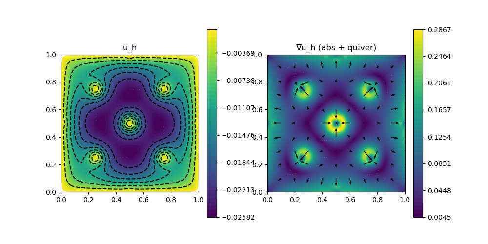
scalarplot!(p[1,1], xgrid, nodevalues_view(Solution[1])[1], levels = 6, title = "u_h")
scalarplot!(p[1,2], xgrid, view(nodevalues(Solution[1], Gradient; abs = true),1,:), levels = 0, colorbarticks = 8, title = "∇u_h (abs + quiver)")
vectorplot!(p[1,2], xgrid, evaluate(PointEvaluator(Solution[1], Gradient)), spacing = 0.1, clear = false)
end
endThis page was generated using Literate.jl.