209 : Lagrange Multiplier on Faces
This code demonstrates the novel feature of finite element spaces on faces by providing AT = ON_FACES in the finite element space constructor. It is used here to solve a bestapproximation into an Hdiv-conforming space by using a broken Hdiv space and setting the normal jumps on interior faces to zero by using a Lagrange multiplier on the faces of the grid (a broken H1-conforming space). Then the solution is compared to the solution of the same problem using the continuous Hdiv-conforming space.
module Example209_FaceLagrangeMultiplier2D
using GradientRobustMultiPhysics
using ExtendableGrids
using GridVisualize
# problem data
function exact_function!(result,x::Array{<:Real,1})
result[1] = x[1]^3+x[2]
result[2] = x[2] + 1
return nothing
end
const u = DataFunction(exact_function!, [2,2]; name = "u", dependencies = "X", bonus_quadorder = 3)
# everything is wrapped in a main function
function main(; Plotter = nothing, verbosity = 0)
# set log level
set_verbosity(verbosity)
# choose initial mesh
xgrid = uniform_refine(grid_unitsquare(Triangle2D),3)
# define bestapproximation problem
Problem = L2BestapproximationProblem(u; name = "constrained L2-bestapproximation problem", bestapprox_boundary_regions = [])
# we want to use a broken space and constrain the normal jumps on interior faces
# in form of a Lagrange multiplier which needs an additional unknown
add_unknown!(Problem; unknown_name = "λ", equation_name = "face jump constraint")
add_operator!(Problem, [1,2], LagrangeMultiplier(NormalFluxDisc{Jump}; AT = ON_IFACES))
# the diagonal operator sets the Lagrange multiplier on all boundary face regions to zero
add_operator!(Problem, [2,2], DiagonalOperator(1; regions = [1,2,3,4]))
@show Problem
# choose some (inf-sup stable) finite element types
# first space is the Hdiv element that lives ON_CELLS
# second will be used for the Lagrange multiplier space that lives ON_FACES
FEType = [HDIVRT1{2}, H1P1{1}]
FES = [FESpace{FEType[1], ON_CELLS}(xgrid; broken = true),FESpace{FEType[2], ON_FACES}(xgrid; broken = true)]
# solve
Solution = solve(Problem, FES)
# solve again with the (unbroken) Hdiv-continuous element to test that we get the same result
# note: for an FESpace living ON_CELLS and broken = false is the default
Problem = L2BestapproximationProblem(u; bestapprox_boundary_regions = [])
Solution2 = FEVector("u_h (Hdiv-cont.)",FESpace{FEType[1]}(xgrid))
solve!(Solution2, Problem)
# calculate L2 error of both solutions and their difference
L2Error = L2ErrorIntegrator(u, Identity)
L2Diff = L2DifferenceIntegrator(2, Identity)
println("\tL2error(Hdiv-broken) = $(sqrt(evaluate(L2Error,Solution[1])))")
println("\tL2error(Hdiv-cont.) = $(sqrt(evaluate(L2Error,Solution2[1])))")
println("\tL2error(difference) = $(sqrt(evaluate(L2Diff,[Solution[1], Solution2[1]])))")
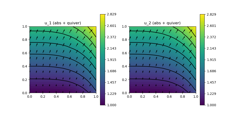
# plot both solutions
p = GridVisualizer(; Plotter = Plotter, layout = (1,2), clear = true, resolution = (1000,500))
scalarplot!(p[1,1],xgrid,view(nodevalues(Solution[1]; abs = true),1,:), levels = 7, title = "u_1 (abs + quiver)")
vectorplot!(p[1,1],xgrid,evaluate(PointEvaluator(Solution[1], Identity)), spacing = 0.1, clear = false)
scalarplot!(p[1,2],xgrid,view(nodevalues(Solution2[1]; abs = true),1,:), levels = 7, title = "u_2 (abs + quiver)")
vectorplot!(p[1,2],xgrid,evaluate(PointEvaluator(Solution2[1], Identity)), spacing = 0.1, clear = false)
end
endThis page was generated using Literate.jl.