221 : Stokes iterated penalty method 2D
This example computes a velocity $\mathbf{u}$ and pressure $\mathbf{p}$ of the incompressible Navier–Stokes problem
\[\begin{aligned} - \mu \Delta \mathbf{u} + (\mathbf{u} \cdot \nabla) \mathbf{u} + \nabla p & = \mathbf{0}\\ \mathrm{div}(u) & = 0 \end{aligned}\]
with some μ parameter $\mu$.
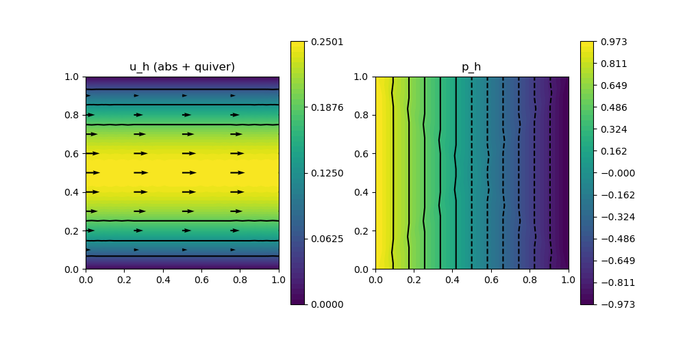
Here we solve the simple Hagen-Poiseuille flow on the two-dimensional unit square domain with the iterated penalty method for the Bernardi–Raugel finite element method. Given intermediate solutions $\mathbf{u}_h$ and $p_h$ the next approximations are computed by the two equations
\[\begin{aligned} (\nabla \mathbf{u}_h^{next}, \nabla \mathbf{v}_h) + ((\mathbf{u}_h^{next} \cdot \nabla) \mathbf{u}_h^{next}, \mathbf{v}_h) + \lambda (\mathrm{div}_h(\mathbf{u}_h) ,\mathrm{div}_h(\mathbf{v}_h)) & = (\mathbf{f},\mathbf{v}_h) + (p_h,\mathrm{div}(\mathbf{v}_h)) && \text{for all } \mathbf{v}_h \in \mathbf{V}_h\\ (p^{next}_h,q_h) & = (p_h,q_h) - \lambda (\mathrm{div}(\mathbf{u}_h^{next}),q_h) && \text{for all } q_h \in Q_h \end{aligned}\]
This is done consecutively until the residual of both equations is small enough. The convection term is linearised by auto-differentiated Newton terms. The discrete divergence is computed via a RT0 reconstruction operator that preserves the disrete divergence. (another way would be to compute Binv(M)B' where M is the mass matrix of the pressure and B is the matrix for the div-pressure block).
module Example221_StokesIterated2D

using GradientRobustMultiPhysics
using ExtendableGrids
using ExtendableSparse
using GridVisualize

# data for Hagen-Poiseuille flow
function exact_pressure!(μ)
    function closure(result,x)
        result[1] = μ*(-2*x[1]+1.0)
    end
end
function exact_velocity!(result,x)
    result[1] = x[2]*(1.0-x[2]);
    result[2] = 0.0;
end

# everything is wrapped in a main function
function main(; verbosity = 0, Plotter = nothing, λ = 1e4, μ = 1.0)

    # set verbosity level
    set_verbosity(verbosity)

    # initial grid
    xgrid = uniform_refine(grid_unitsquare(Triangle2D), 4)

    # Bernardi--Raugel element
    FETypes = [H1BR{2}, L2P0{1}]; PenaltyDivergence = ReconstructionDivergence{HDIVRT0{2}}

    # FE spaces
    FES = [FESpace{FETypes[1]}(xgrid), FESpace{FETypes[2]}(xgrid; broken = true)]

    # negotiate data functions to the package
    u = DataFunction(exact_velocity!, [2,2]; name = "u", dependencies = "X", bonus_quadorder = 2)
    p = DataFunction(exact_pressure!(μ), [1,2]; name = "p", dependencies = "X", bonus_quadorder = 1)

    # generate Stokes problem
    Problem = PDEDescription("NSE (iterated penalty)")
    add_unknown!(Problem; equation_name = "velocity update", unknown_name = "u")
    add_unknown!(Problem; equation_name = "pressure update", unknown_name = "p")
    add_constraint!(Problem, FixedIntegralMean(2,0))

    # add boundary data
    add_boundarydata!(Problem, 1, [1,2,3,4], InterpolateDirichletBoundary; data = u)

    # velocity update equation
    add_operator!(Problem, [1,1], LaplaceOperator(μ; store = true))
    add_operator!(Problem, [1,2], BilinearForm([Divergence, Identity]; store = false, factor = -1))
    add_operator!(Problem, [1,1], ConvectionOperator(1, Identity, 2, 2; newton = false))

    # add penalty for discrete divergence
    add_operator!(Problem, [1,1], BilinearForm([PenaltyDivergence, PenaltyDivergence]; store = true, factor = λ))

    # pressure update equation
    add_operator!(Problem, [2,2], BilinearForm([Identity, Identity]; store = false))
    rhs_action = Action((result,input) -> (result[1] = input[1] - λ*input[2]), [1, 3])
    add_rhsdata!(Problem, 2, LinearForm(Identity, [Identity, Divergence], [2, 1], rhs_action; name = "(#1 - λdiv(#2), #T)"))

    # show and solve problem
    @show Problem
    Solution = FEVector([FES[1],FES[2]])
    solve!(Solution, Problem; subiterations = [[1],[2]], maxiterations = 20, show_solver_config = true, show_statistics = true)

    # calculate L2 error
    L2ErrorV = L2ErrorIntegrator(u, Identity)
    L2ErrorP = L2ErrorIntegrator(p, Identity)
    println("|| u - u_h || = $(sqrt(evaluate(L2ErrorV,Solution[1])))")
    println("|| p - p_h || = $(sqrt(evaluate(L2ErrorP,Solution[2])))")

    # plot
    p = GridVisualizer(; Plotter = Plotter, layout = (1,2), clear = true, resolution = (1000,500))
    scalarplot!(p[1,1],xgrid,view(nodevalues(Solution[1]; abs = true),1,:), levels = 3)
    vectorplot!(p[1,1],xgrid,evaluate(PointEvaluator(Solution[1], Identity)), spacing = [0.25,0.1], clear = false, title = "u_h (abs + quiver)")
    scalarplot!(p[1,2],xgrid,view(nodevalues(Solution[2]),1,:), levels = 11, title = "p_h")
end
end
This page was generated using Literate.jl.