225 : Navier-Stokes Lid-driven cavity + Anderson Acceleration
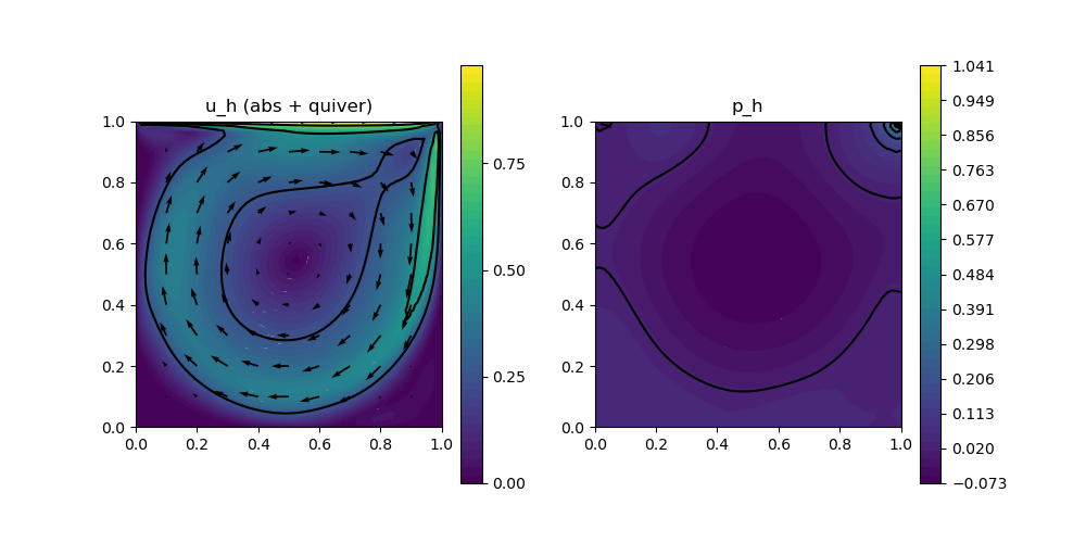
This example solves the lid-driven cavity problem where one seeks a velocity $\mathbf{u}$ and pressure $\mathbf{p}$ of the incompressible Navier–Stokes problem
\[\begin{aligned} - \mu \Delta \mathbf{u} + (\mathbf{u} \cdot \nabla) \mathbf{u} + \nabla p & = 0\\ \mathrm{div}(u) & = 0 \end{aligned}\]
where $\mathbf{u} = (1,0)$ along the top boundary of a square domain.
For small viscosities (where a Newton and a classical Picard iteration do not converge anymore), Anderson acceleration might help which can be tested with this script. Here, we use Anderson acceleration until the residual is small enough for the Newton to take over.
module Example225_NavierStokesAnderson2D

using GradientRobustMultiPhysics
using ExtendableGrids
using GridVisualize
using Printf

# everything is wrapped in a main function
function main(; verbosity = 0, Plotter = nothing, μ = 5e-4, anderson_iterations = 10, target_residual = 1e-12, maxiterations = 50, switch_to_newton_tolerance = 1e-4)

    # set log level
    set_verbosity(verbosity)

    # grid
    xgrid = uniform_refine(grid_unitsquare(Triangle2D), 5);

    # finite element type
    FETypes = [H1P2{2,2}, H1P1{1}] # Taylor--Hood

    # load Navier-Stokes problem prototype and assign data
    Problem = IncompressibleNavierStokesProblem(2; viscosity = μ, nonlinear = true, newton = false, store = false)
    add_boundarydata!(Problem, 1, [1,2,4], HomogeneousDirichletBoundary)
    add_boundarydata!(Problem, 1, [3], BestapproxDirichletBoundary; data = DataFunction([1,0]))
    @show Problem

    # generate FESpaces
    FES = [FESpace{FETypes[1]}(xgrid), FESpace{FETypes[2]}(xgrid)]
    Solution = FEVector(FES)

    # solve with anderson iterations until 1e-4
    solve!(Solution, Problem; anderson_iterations = anderson_iterations, anderson_metric = "l2", anderson_unknowns = [1], maxiterations = maxiterations, target_residual = switch_to_newton_tolerance, show_statistics = true)

    # solve rest with Newton
    Problem = IncompressibleNavierStokesProblem(2; viscosity = μ, nonlinear = true, newton = true, store = true)
    add_boundarydata!(Problem, 1, [1,2,4], HomogeneousDirichletBoundary)
    add_boundarydata!(Problem, 1, [3], BestapproxDirichletBoundary; data = DataFunction([1,0]))
    @show Problem
    solve!(Solution, Problem; anderson_iterations = anderson_iterations, maxiterations = maxiterations, target_residual = target_residual, show_statistics = true)

    # plot
    p = GridVisualizer(; Plotter = Plotter, layout = (1,2), clear = true, resolution = (1000,500))
    scalarplot!(p[1,1],xgrid,view(nodevalues(Solution[1]; abs = true),1,:), levels = 3)
    vectorplot!(p[1,1],xgrid,evaluate(PointEvaluator(Solution[1], Identity)), spacing = 0.1, clear = false, title = "u_h (abs + quiver)")
    scalarplot!(p[1,2],xgrid,view(nodevalues(Solution[2]),1,:), levels = 11, title = "p_h")
end

end
This page was generated using Literate.jl.