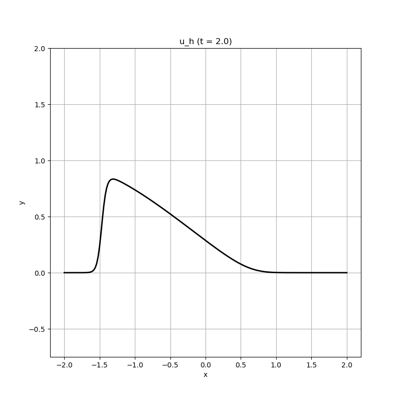
103 : Burger's Equation 1D
This example solves the Burger's equation
\[\begin{aligned} u_t - \mu \Delta u + \mathrm{div} f(u) & = 0 \end{aligned}\]
with periodic boundary conditions.
module Example103_BurgersEquation1D

using GradientRobustMultiPhysics
using ExtendableGrids
using GridVisualize

const f = (result, u) -> (result[1] = u[1]^2/2;) # kernel for nonlinearity
const u0 = DataFunction((result,x) -> (result[1] = abs(x[1]) < 0.5 ? 1 : 0), [1, 1]; dependencies = "X", bonus_quadorder = 4)     # initial height

# everything is wrapped in a main function
function main(; verbosity = 0, ν = 1e-2, h = 0.02, T = 2, order = 2, τ = 5//100, Plotter = nothing)

    # set log level
    set_verbosity(verbosity)

    # load mesh and exact solution
    xgrid = simplexgrid(-2:h:2)

    # set finite element types [surface height, velocity]
    FEType = H1Pk{1,1,order}

    # generate empty PDEDescription for three unknowns (h, u)
    Problem = PDEDescription("Burger's Equation")
    add_unknown!(Problem; unknown_name = "u", equation_name = "Burger's Equation")
    add_operator!(Problem, 1, NonlinearForm(Gradient, [Identity], [1], f, [1,1]; name = "(f(#A),∇#T)", newton = true, bonus_quadorder = 2))
    add_operator!(Problem, [1,1], LaplaceOperator(ν))
    add_constraint!(Problem, CombineDofs(1, 1, [1],[num_nodes(xgrid)]))
    @show Problem

    # prepare solution vector and interpolate u0
    Solution = FEVector("u_h", FESpace{FEType}(xgrid))
    interpolate!(Solution[1], u0)

    # init plotter and plot u0
    p = GridVisualizer(; Plotter = Plotter, layout = (1,1), clear = true, resolution = (800,800))
    scalarplot!(p[1,1], xgrid, nodevalues_view(Solution[1])[1], flimits = (-0.75,2), levels = 0, title = "u_h (t = 0)")

    # configure time-dependent solver
    TCS = TimeControlSolver(Problem, Solution, BackwardEuler;
                                        timedependent_equations = [1],
                                        maxiterations = 10,
                                        show_iteration_details = true,
                                        T_time = typeof(τ))

    # advance in time
    function do_each_timestep(kwargs...)
        scalarplot!(p[1,1], xgrid, nodevalues_view(Solution[1])[1], flimits = (-0.75,2), levels = 0, title = "u_h (t = $(Float64(TCS.ctime)))")
    end
    advance_until_time!(TCS, τ, T; do_after_each_timestep = do_each_timestep)
end
end
This page was generated using Literate.jl.