102 : Robin-Boundary Conditions 1D
This demonstrates the assignment of a mixed Robin boundary condition for a nonlinear 1D convection-diffusion-reaction PDE on the unit interval, i.e.
\[\begin{aligned} -\partial^2 u / \partial x^2 + u \partial u / \partial x + u & = f && \text{in } \Omega\\ u + \partial u / \partial_x & = g && \text{at } \Gamma_1 = \{ 0 \}\\ u & = u_D && \text{at } \Gamma_2 = \{ 1 \} \end{aligned}\]
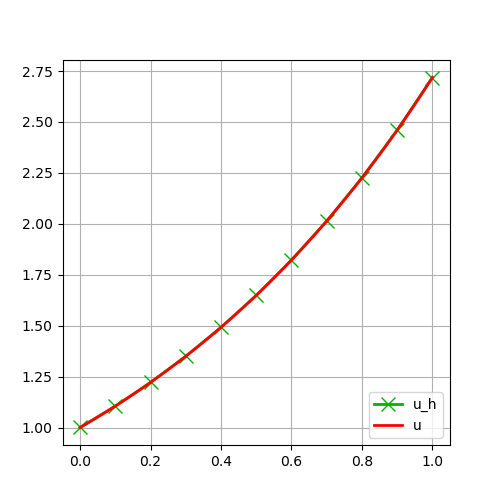
tested with data $f(x) = e^{2x}$, $g = 2$ and $u_D = e$ such that $u(x) = e^x$ is the exact solution.
module Example102_RobinBoundaryCondition1D

using GradientRobustMultiPhysics
using ExtendableGrids
using GridVisualize

# data and exact solution
const f = DataFunction((result,x) -> (result[1] = exp(2*x[1]);), [1,1]; name = "f", dependencies = "X", bonus_quadorder = 4)
const u = DataFunction((result,x) -> (result[1] = exp(x[1]);), [1,1]; name = "u", dependencies = "X", bonus_quadorder = 4)
const g = DataFunction([2]; name = "g")
const uD = DataFunction([exp(1)]; name = "u_D")

# kernel for the (nonlinear) reaction-convection-diffusion oeprator
function operator_kernel!(result, input)
    # input = [u,∇u] as a vector of length 2
    result[1] = input[1] * input[2] + input[1] # convection + reaction (will be multiplied with v)
    result[2] = input[2]                       # diffusion (will be multiplied with ∇v)
    return nothing
end

# kernel for Robin boundary condition
function robin_kernel!(result, input)
    # input = [u]
    result[1] = g()[1] - input[1] # = g - u (will be multiplied with v)
    return nothing
end

# everything is wrapped in a main function
function main(; Plotter = nothing, verbosity = 0, h = 1e-1, h_fine = 1e-3)

    # set log level
    set_verbosity(verbosity)

    # generate coarse and fine mesh
    xgrid = simplexgrid(0:h:1)

    # setup a problem description with one unknown
    Problem = PDEDescription("reaction-convection-diffusion problem")
    add_unknown!(Problem; unknown_name = "u", equation_name = "reaction-convection-diffusion equation")

    # add nonlinear operator
    add_operator!(Problem, [1,1], NonlinearForm(OperatorPair{Identity, Gradient}, [OperatorPair{Identity, Gradient}], [1], operator_kernel!, [2,2]; name = "(∇#1, ∇#T) + (#1∇#1 + #1, #T)", bonus_quadorder = 4, newton = true) )

    # right-hand side data
    add_rhsdata!(Problem, 1, LinearForm(Identity, f))

    # Robin boundary data right
    add_operator!(Problem, [1,1], BilinearForm([Identity, Identity], Action(robin_kernel!, [1,1]); name = "(g - #A, #T)", AT = ON_BFACES, regions = [1]) )

    # Dirichlet boundary data left
    add_boundarydata!(Problem, 1, [2], InterpolateDirichletBoundary; data = uD)

    @show Problem

    # choose some finite element type and generate a FESpace for the grid
    # (here it is a one-dimensional H1-conforming P2 element H1P2{1,1})
    FEType = H1P2{1,1}
    FES = FESpace{FEType}(xgrid)

    # generate a solution vector and solve
    Solution = solve(Problem, FES; show_statistics = true)

    # compute L2 error
    L2error = L2ErrorIntegrator(u)
    println("L2error = $(sqrt(evaluate(L2error,Solution[1])))")

    # plot discrete and exact solution (on finer grid)
    p=GridVisualizer(Plotter = Plotter, layout = (1,1))
    scalarplot!(p[1,1], xgrid, nodevalues_view(Solution[1])[1], color=(0,0.7,0), label = "u_h", markershape = :x, markersize = 10, markevery = 1)
    xgrid_fine = simplexgrid(0:h_fine:1)
    scalarplot!(p[1,1], xgrid_fine, view(nodevalues(xgrid_fine,u),1,:), clear = false, color = (1,0,0), label = "u", legend = :rb, markershape = :none)
end

end
This page was generated using Literate.jl.