224 : Stokes $SV + RT enrichment$

(source code)

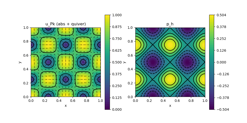
This example computes the velocity $\mathbf{u}$ and pressure $\mathbf{p}$ of the incompressible Navier–Stokes problem

\[\begin{aligned} - \mu \Delta \mathbf{u} + \nabla p & = \mathbf{f}\\ \mathrm{div}(u) & = 0 \end{aligned}\]

with exterior force $\mathbf{f}$ and some parameter $\mu$ and inhomogeneous Dirichlet boundary data.

The problem will be solved by a $(P_k \oplus RTenrichment) \times P_{k-1}$ scheme, which can be seen as an inf-sup stabilized Scott-Vogelius variant, see references below. Therein, the velocity space employs continuous Pk functions plus certain (only H(div)-conforming) Raviart-Thomas functions and a discontinuous Pk-1 pressure space leading to an exactly divergence-free discrete velocity.

module Example224_StokesSVRTEnrichment

using GradientRobustMultiPhysics
using ExtendableGrids
using GridVisualize
using SimplexGridFactory
using Triangulate

# flow data for boundary condition, right-hand side and error calculation
function get_flowdata(ν, nonlinear)
    u = DataFunction((result, x, t) -> (
            result[1] = exp(-8*pi*pi*ν*t)*sin(2*pi*x[1])*sin(2*pi*x[2]);
            result[2] = exp(-8*pi*pi*ν*t)*cos(2*pi*x[1])*cos(2*pi*x[2]);
        ), [2,2]; name = "u", dependencies = "XT", bonus_quadorder = 6)
    p = DataFunction((result, x, t) -> (
            result[1] = exp(-8*pi*pi*ν*t)*(cos(4*pi*x[1])-cos(4*pi*x[2])) / 4
        ), [1,2]; name = "p", dependencies = "XT", bonus_quadorder = 4)
    Δu = Δ(u)
    ∇p = ∇(p)
    f = DataFunction((result, x, t) -> (
            result .= -ν * Δu(x,t);
            if !nonlinear
                result .+= ∇p(x,t);
            end;
        ), [2,2]; name = "f", dependencies = "XT", bonus_quadorder = 6)
    return u, p, ∇(u), f
end

# everything is wrapped in a main function
function main(; μ = 1e-3, nlevels = 4, Plotter = nothing, order = 2, verbosity = 0, T = 0)

    # set log level
    set_verbosity(verbosity)

    # FEType Pk + enrichment + pressure
    @assert order in 1:4
    if order == 1
        FETypes = [H1P1{2}, HDIVRT0{2}, L2P0{1}]
    else
        FETypes = [H1Pk{2,2,order}, HDIVRTkENRICH{2, order-1}, H1Pk{1,2,order-1}]
    end

    # get exact flow data (see above)
    u,p,∇u,f = get_flowdata(μ, false)

    # generate and show problem description
    Problem = get_problem(; order = order, μ = μ, rhs = f, boundary_data = u)
    @show Problem

    # prepare error calculation
    L2VelocityError = L2ErrorIntegrator(u, [Identity, Identity]; time = T)
    L2PressureError = L2ErrorIntegrator(p, Identity; time = T)
    H1VelocityError = L2ErrorIntegrator(∇u, Gradient; time = T)
    L2NormR = L2NormIntegrator(2 , [Identity])
    L2VeloDivEvaluator = L2NormIntegrator(1 , [Divergence, Divergence])
    Results = zeros(Float64,nlevels,5); NDofs = zeros(Int,nlevels)

    # loop over levels
    Solution = nothing
    xgrid = nothing
    for level = 1 : nlevels
        # generate unstructured grid
        xgrid = simplexgrid(Triangulate;
                    points=[0 0 ; 0 1 ; 1 1 ; 1 0]',
                    bfaces=[1 2 ; 2 3 ; 3 4 ; 4 1 ]',
                    bfaceregions=[1, 2, 3, 4],
                    regionpoints=[0.5 0.5;]',
                    regionnumbers=[1],
                    regionvolumes=[4.0^(-level-1)/2])

        # generate FES spaces and solution vector
        FES = [FESpace{FETypes[1]}(xgrid), FESpace{FETypes[2]}(xgrid), FESpace{FETypes[3]}(xgrid; broken = true)]
        Solution = FEVector(FES)

        # solve
        solve!(Solution, Problem; time = T)

        # compute L2 and H1 errors and save data
        NDofs[level] = length(Solution.entries)
        Results[level,1] = sqrt(evaluate(L2VelocityError,[Solution[1], Solution[2]]))
        Results[level,2] = sqrt(evaluate(L2PressureError,Solution[3]))
        Results[level,3] = sqrt(evaluate(H1VelocityError,Solution[1]))
        Results[level,4] = sqrt(evaluate(L2NormR,Solution[2]))
        Results[level,5] = sqrt(evaluate(L2VeloDivEvaluator,[Solution[1], Solution[2]]))
    end

    # plot
    p = GridVisualizer(; Plotter = Plotter, layout = (1,2), clear = true, resolution = (1000,500))
    scalarplot!(p[1,1],xgrid,view(nodevalues(Solution[1]; abs = true),1,:), levels = 3, colorbarticks = 9, title = "u_Pk (abs + quiver)")
    vectorplot!(p[1,1],xgrid,evaluate(PointEvaluator(Solution[1], Identity)), spacing = 0.05, clear = false)
    scalarplot!(p[1,2],xgrid,view(nodevalues(Solution[3]),1,:), levels = 7, title = "p_h")

    # print convergence history
    print_convergencehistory(NDofs, Results; X_to_h = X -> X.^(-1/2), ylabels = ["|| u - u_h ||", "|| p - p_h ||", "|| ∇(u - u_P1) ||", "|| u_R ||", "|| div(u_h) ||"])
end

function get_problem(; μ = 1, order = 1, boundary_data = nothing, rhs = nothing)
    # define problem
    Problem = PDEDescription("Stokes problem")
    add_unknown!(Problem; equation_name = "momentum equation (Pk part)", unknown_name = "u_Pk")
    add_unknown!(Problem; equation_name = "momentum equation (RT enrichment)", unknown_name = "u_RT")
    add_unknown!(Problem; equation_name = "incompressibility constraint", unknown_name = "p")

    # add Laplacian for Pk part
    add_operator!(Problem, [1,1], LaplaceOperator(μ))

    if order > 1 ## add consistency terms (skew-symmetric)
        add_operator!(Problem, [1,2], BilinearForm([Laplacian, Identity]; factor = μ, also_transposed_block = true, transpose_factor = -μ))
    else ## add stabilisation for RT0
        α = 1.0
        lump = true
        ARR = BilinearForm([Divergence, Divergence]; factor = α*μ, APT = lump ? APT_LumpedBilinearForm : APT_BilinearForm)
        add_operator!(Problem, [2,2], ARR)
    end

    # add Lagrange multiplier for divergence of velocity
    add_operator!(Problem, [1,3], LagrangeMultiplier(Divergence))
    add_operator!(Problem, [2,3], LagrangeMultiplier(Divergence))
    add_constraint!(Problem, FixedIntegralMean(3,0))

    # add boundary data and right-hand side
    if boundary_data !== nothing
        add_boundarydata!(Problem, 1, [1,2,3,4], InterpolateDirichletBoundary; data = boundary_data)
        if order == 1
            add_boundarydata!(Problem, 2, [1,2,3,4], CorrectDirichletBoundary{1}; data = boundary_data) # <- RT part corrects (piecewise normal flux integrals of) P1 part
        end
    else
        add_boundarydata!(Problem, 1, [1,2,3,4], HomogeneousDirichletBoundary)
        if order == 1
            add_boundarydata!(Problem, 2, [1,2,3,4], HomogeneousDirichletBoundary)
        end
    end
    if rhs !== nothing
        add_rhsdata!(Problem, 1, LinearForm(Identity, rhs))
        add_rhsdata!(Problem, 2, LinearForm(Identity, rhs))
    end
    return Problem
end


# test function that is called by test unit
# tests if polynomial solution is computed exactly
function test(; μ = 1e-3)
    maxerror = 0
    for order = 1 : 4
        # generate test data
        u = DataFunction((result, x) -> (
                result[1] = x[2]*(1-x[2])^(order-1) + 1 + x[2] - x[1];
                result[2] = x[1]*(1-x[1])^(order-1) - 1 - x[1] + x[2];
            ), [2,2]; name = "u", dependencies = "X", bonus_quadorder = order)
        p = DataFunction((result, x) -> (
                result[1] = x[1]^4 + x[2]^4 - 2//5
            ), [1,2]; name = "p", dependencies = "X", bonus_quadorder = 4)
        Δu = Δ(u)
        ∇p = ∇(p)
        f = DataFunction((result, x) -> (
                result .= -μ * Δu(x) .+ ∇p(x);
            ), [2,2]; name = "f", dependencies = "X", bonus_quadorder = 6)


        # generate unstructured grid
        xgrid = simplexgrid(Triangulate;
                    points=[0 0 ; 0 1 ; 1 1 ; 1 0]',
                    bfaces=[1 2 ; 2 3 ; 3 4 ; 4 1 ]',
                    bfaceregions=[1, 2, 3, 4],
                    regionpoints=[0.5 0.5;]',
                    regionnumbers=[1],
                    regionvolumes=[1.0/8])

        # generate FES spaces and solution vector
        if order == 1
            FETypes = [H1P1{2}, HDIVRT0{2}, L2P0{1}]
        else
            FETypes = [H1Pk{2,2,order}, HDIVRTkENRICH{2, order-1}, H1Pk{1,2,order-1}]
        end
        FES = [FESpace{FETypes[1]}(xgrid), FESpace{FETypes[2]}(xgrid), FESpace{FETypes[3]}(xgrid; broken = true)]
        Solution = FEVector(FES)

        # solve
        Problem = get_problem(; order = order, μ = μ, rhs = f, boundary_data = u)
        solve!(Solution, Problem)

        L2VelocityError = L2ErrorIntegrator(u, [Identity, Identity])
        L2VeloDivEvaluator = L2NormIntegrator(1, [Divergence, Divergence])
        errorL2 = sqrt(evaluate(L2VelocityError, [Solution[1], Solution[2]]))
        errorL2div = sqrt(evaluate(L2VeloDivEvaluator, [Solution[1], Solution[2]]))

        @show order, errorL2, errorL2div
        maxerror = max(errorL2 + errorL2div, maxerror)
    end

    return maxerror
end

end

This page was generated using Literate.jl.