222 : Pressure-robustness 2D
This example studies two benchmarks for pressure-robust discretisations of the stationary Navier-Stokes equations that seek a velocity $\mathbf{u}$ and pressure $\mathbf{p}$ such that
\[\begin{aligned} - \mu \Delta \mathbf{u} + (\mathbf{u} \cdot \nabla) \mathbf{u} + \nabla p & = \mathbf{f}\\ \mathrm{div}(u) & = 0 \end{aligned}\]
with (possibly time-dependent) exterior force $\mathbf{f}$ and some viscosity parameter $\mu$.
Pressure-robustness is concerned with gradient forces that may appear in the right-hand side or the material derivative and should be balanced by the pressure (as divergence-free vector fields are orthogonal on gradient fields). Here, two test problems are considered:
- HydrostaticTestProblem() : Stokes (without convection term) and $\mathbf{f} = \nabla p$ such that $\mathbf{u} = 0$
- PotentialFlowTestProblem() : Navier-Stokes with $\mathbf{f} = 0$ and $\mathbf{u} = \nabla h$ for some harmonic function
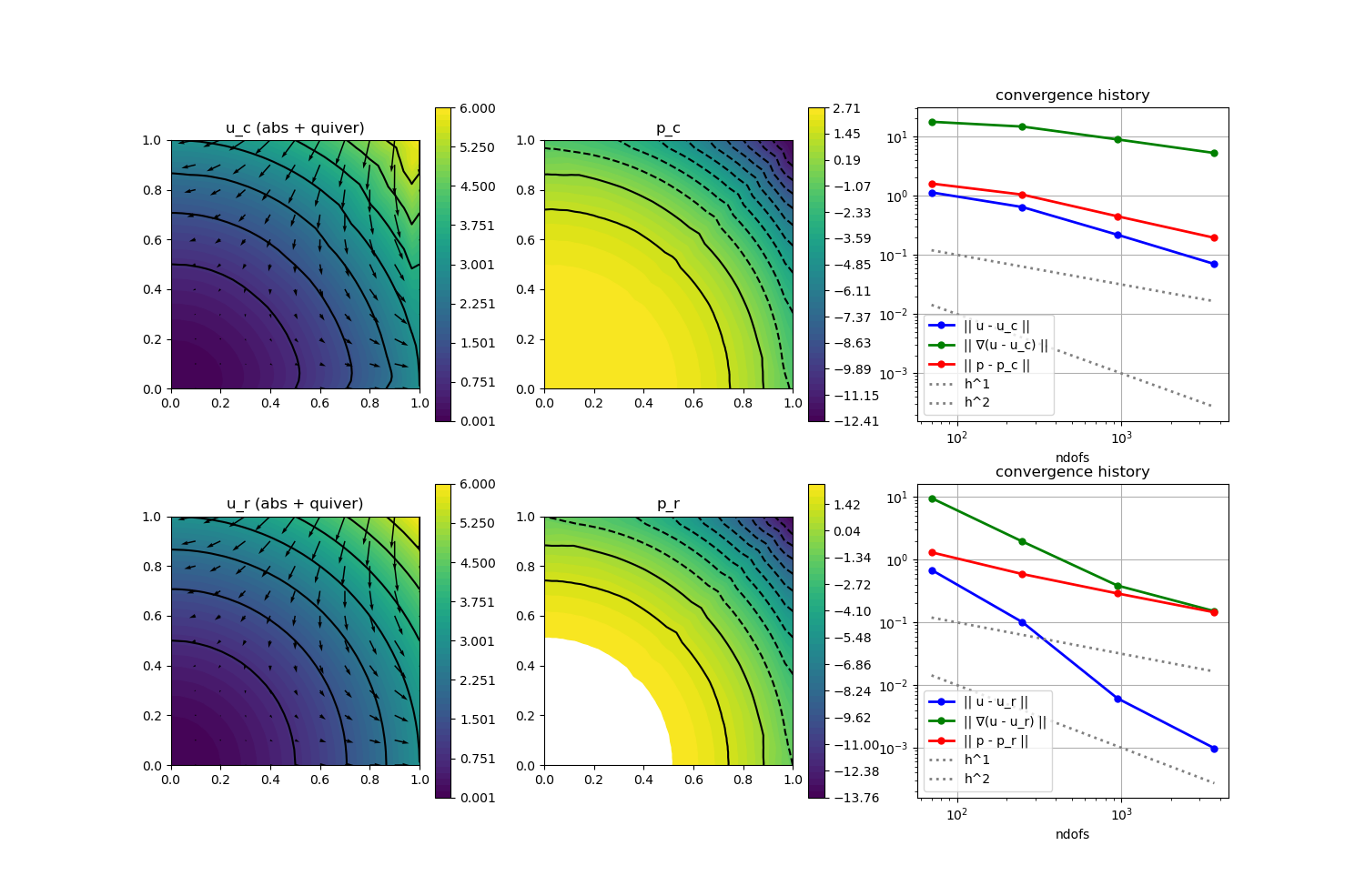
In both test problems the errors of non-pressure-robust discretisations scale with $1/\mu$, while the pressure-robust discretisation solves $\mathbf{u} = 0$ exactly in test problem 1 and gives much better results in test problem 2.
module Example222_PressureRobustness2D

using GradientRobustMultiPhysics
using ExtendableGrids
using GridVisualize

# problem data
function HydrostaticTestProblem()
    # Stokes problem with f = grad(p)
    # u = 0,  p = x^3+y^3 - 1//2
    function P1_pressure!(result,x)
        result[1] = x[1]^3 + x[2]^3 - 1//2
    end
    u = DataFunction([0,0]; xdim = 2, name = "u")
    p = DataFunction(P1_pressure!, [1,2]; name = "p", dependencies = "X", bonus_quadorder = 3)
    f = ∇(p)
    return p,u,∇(u),f,false
end

function PotentialFlowTestProblem()
    # NavierStokes with f = 0
    # u = grad(h) with h = x^3 - 3xy^2
    # p = - |grad(h)|^2 + 14//5
    function P2_pressure!(result,x)
        result[1] = - 1//2 * (9*(x[1]^4 + x[2]^4) + 18*x[1]^2*x[2]^2) + 14//5
    end
    function P2_velo!(result,x)
        result[1] = 3*x[1]^2 - 3*x[2]^2;
        result[2] = -6*x[1]*x[2];
    end
    u = DataFunction(P2_velo!, [2,2]; name = "u", dependencies = "X", bonus_quadorder = 2)
    p = DataFunction(P2_pressure!, [1,2]; name = "p", dependencies = "X", bonus_quadorder = 4)
    f = DataFunction([0,0]; name = "f")
    return p,u,∇(u),f,true
end


function solver(Problem, xgrid, FETypes, viscosity = 1e-2; nlevels = 4, target_residual = 1e-10, maxiterations = 20, Plotter = nothing)

    # load problem data and set solver parameters
    ReconstructionOperator = FETypes[3]
    p,u,∇u,f,nonlinear = Problem()

    # setup classical (Problem) and pressure-robust scheme (Problem2)
    Problem = IncompressibleNavierStokesProblem(2; viscosity = viscosity, nonlinear = false)
    add_boundarydata!(Problem, 1, [1,2,3,4], BestapproxDirichletBoundary; data = u)
    Problem2 = deepcopy(Problem)
    Problem.name = "Stokes problem (classical)"
    Problem2.name = "Stokes problem (p-robust)"

    # assign right-hand side
    add_rhsdata!(Problem, 1, LinearForm(Identity, f))
    add_rhsdata!(Problem2, 1, LinearForm(ReconstructionOperator, f))

    # assign convection term
    if nonlinear
        add_operator!(Problem,[1,1], ConvectionOperator(1, Identity, 2, 2))
        add_operator!(Problem2,[1,1], ConvectionOperator(1, ReconstructionOperator, 2, 2; test_operator = ReconstructionOperator))
    end

    # define bestapproximation problems
    BAP_L2_u = L2BestapproximationProblem(u; bestapprox_boundary_regions = [1,2,3,4])
    BAP_L2_p = L2BestapproximationProblem(p; bestapprox_boundary_regions = [])
    BAP_H1_u = H1BestapproximationProblem(∇u, u; bestapprox_boundary_regions = [1,2,3,4])

    # define ItemIntegrators for L2/H1 error computation
    L2Error_u = L2ErrorIntegrator(u, Identity)
    L2Error_p = L2ErrorIntegrator(p, Identity)
    H1Error_u = L2ErrorIntegrator(∇u, Gradient)
    Results = zeros(Float64, nlevels, 9)
    NDofs = zeros(Int, nlevels)

    # loop over refinement levels
    Solution, Solution2 = nothing, nothing
    for level = 1 : nlevels

        # uniform mesh refinement
        xgrid = uniform_refine(xgrid)

        # get FESpaces
        FES = [FESpace{FETypes[1]}(xgrid), FESpace{FETypes[2]}(xgrid; broken = true)]

        # solve both problems
        Solution = solve(Problem, FES; maxiterations = maxiterations, target_residual = target_residual, anderson_iterations = 5)
        Solution2 = solve(Problem2, FES; maxiterations = maxiterations, target_residual = target_residual, anderson_iterations = 5)

        # solve bestapproximation problems
        BA_L2_u = FEVector("Πu",FES[1])
        BA_L2_p = FEVector("πp",FES[2])
        BA_H1_u = FEVector("Su",FES[1])
        solve!(BA_L2_u, BAP_L2_u)
        solve!(BA_L2_p, BAP_L2_p)
        solve!(BA_H1_u, BAP_H1_u)

        # compute L2 and H1 errors and save data
        NDofs[level] = length(Solution.entries)
        Results[level,1] = sqrt(evaluate(L2Error_u,Solution[1]))
        Results[level,2] = sqrt(evaluate(L2Error_u,Solution2[1]))
        Results[level,3] = sqrt(evaluate(L2Error_u,BA_L2_u[1]))
        Results[level,4] = sqrt(evaluate(L2Error_p,Solution[2]))
        Results[level,5] = sqrt(evaluate(L2Error_p,Solution2[2]))
        Results[level,6] = sqrt(evaluate(L2Error_p,BA_L2_p[1]))
        Results[level,7] = sqrt(evaluate(H1Error_u,Solution[1]))
        Results[level,8] = sqrt(evaluate(H1Error_u,Solution2[1]))
        Results[level,9] = sqrt(evaluate(H1Error_u,BA_H1_u[1]))
    end

    # print convergence history
    print_convergencehistory(NDofs, Results[:,1:3]; X_to_h = X -> X.^(-1/2), ylabels = ["||u-u_c||", "||u-u_r||", "||u-Πu||"])
    print_convergencehistory(NDofs, Results[:,4:6]; X_to_h = X -> X.^(-1/2), ylabels = ["||p-p_c||", "||p-p_r||", "||p-πp||"])
    print_convergencehistory(NDofs, Results[:,7:9]; X_to_h = X -> X.^(-1/2), ylabels = ["||∇(u-u_c)||", "||∇(u-u_r)||", "||∇(u-Su)||"])

    # plot
    p = GridVisualizer(; Plotter = Plotter, layout = (2,3), clear = true, resolution = (1500,1000))
    scalarplot!(p[1,1],xgrid,view(nodevalues(Solution[1]; abs = true),1,:), levels = 7)
    vectorplot!(p[1,1],xgrid,evaluate(PointEvaluator(Solution[1], Identity)), spacing = 0.1, clear = false, title = "u_c (abs + quiver)")
    scalarplot!(p[1,2],xgrid,view(nodevalues(Solution[2]),1,:), levels = 11, title = "p_c")
    scalarplot!(p[2,1],xgrid,view(nodevalues(Solution2[1]; abs = true),1,:), levels = 7)
    vectorplot!(p[2,1],xgrid,evaluate(PointEvaluator(Solution2[1], Identity)), spacing = 0.1, clear = false, title = "u_r (abs + quiver)")
    scalarplot!(p[2,2],xgrid,view(nodevalues(Solution2[2]),1,:), levels = 11, title = "p_r")
    convergencehistory!(p[1,3], NDofs, Results[:,[1,7,4]]; add_h_powers = [1,2], X_to_h = X -> X.^(-1/2), ylabels = ["|| u - u_c ||", "|| ∇(u - u_c) ||", "|| p - p_c ||"])
    convergencehistory!(p[2,3], NDofs, Results[:,[2,8,5]]; add_h_powers = [1,2], X_to_h = X -> X.^(-1/2), ylabels = ["|| u - u_r ||", "|| ∇(u - u_r) ||", "|| p - p_r ||"])

    # return last L2 error of p-robust method for testing
    return Results[end,2]
end


# everything is wrapped in a main function
function main(; problem = 2, verbosity = 0, nlevels = 4, viscosity = 1e-2, Plotter = nothing)

    # set log level
    set_verbosity(verbosity)

    # set problem to solve
    if problem == 1
        Problem = HydrostaticTestProblem
    elseif problem == 2
        Problem = PotentialFlowTestProblem
    else
        @error "No problem defined for this number!"
    end

    # set grid and problem parameters
    xgrid = grid_unitsquare(Triangle2D) # initial grid

    # choose finite element discretisation
    #FETypes = [H1BR{2}, L2P0{1}, ReconstructionIdentity{HDIVRT0{2}}] # Bernardi--Raugel with RT0 reconstruction
    FETypes = [H1BR{2}, L2P0{1}, ReconstructionIdentity{HDIVBDM1{2}}] # Bernardi--Raugel with BDM1 reconstruction
    #FETypes = [H1CR{2}, L2P0{1}, ReconstructionIdentity{HDIVRT0{2}}] # Crouzeix--Raviart with RT0 reconstruction

    # run
    solver(Problem, xgrid, FETypes, viscosity; nlevels = nlevels, Plotter = Plotter)

    return nothing
end


# test function that is called by test unit
# tests if hydrostatic problem is solved exactly by pressure-robust methods
function test(; Plotter = nothing)
    xgrid = uniform_refine(grid_unitsquare_mixedgeometries())
    testspaces = [[H1CR{2}, L2P0{1}, ReconstructionIdentity{HDIVRT0{2}}],
                  [H1BR{2}, L2P0{1}, ReconstructionIdentity{HDIVRT0{2}}],
                  [H1BR{2}, L2P0{1}, ReconstructionIdentity{HDIVBDM1{2}}]
                  ]
    error = []
    for FETypes in testspaces
        push!(error, solver(HydrostaticTestProblem, xgrid, FETypes, 1; nlevels = 1))
        println("FETypes = $FETypes   error = $(error[end])")
    end

    xgrid = uniform_refine(grid_unitsquare(Triangle2D))
    testspaces = [
                  [H1P2B{2,2}, H1P1{1}, ReconstructionIdentity{HDIVRT1{2}}]
                  ]
    error = []
    for FETypes in testspaces
        push!(error, solver(HydrostaticTestProblem, xgrid, FETypes, 1; nlevels = 1, Plotter = Plotter))
        println("FETypes = $FETypes   error = $(error[end])")
    end
    return maximum(error)
end

end
This page was generated using Literate.jl.