212 : Wave Equation 2D
This example computes the transient solution of the wave equation
\[\frac{\partial^2 u}{\partial t^2} = c \Delta u + f\]
with propagation speed $c$ and source term $f$.
The equation can be rewritten into the system of two PDEs
\[\begin{aligned} u_t & = v\\ v_t & = c \Delta u + f. \end{aligned}\]
Here, we solve the equations on a circle domain with $c = 1$ and $f = 0$ for some given initial state and homogeneous Dirichlet boundary conditions.
module Example212_WaveEquation2D
using GradientRobustMultiPhysics
using ExtendableGrids
using GridVisualize
using SimplexGridFactory
using Triangulate
const u0 = DataFunction((result,x) -> (result[1] = 1 - x[1]^2 - x[2]^2), [1,2]; dependencies = "X", bonus_quadorder = 2)
const v0 = DataFunction([0.0])
const f = DataFunction([0.0])
const c = 1
# everything is wrapped in a main function
function main(; verbosity = 0, order = 1, reflevel = 2, T = 0.65, timestep = 1//100, plot_step = 1//20, Plotter = nothing)
# set log level
set_verbosity(verbosity)
# initial grid and final time
xgrid = grid_circle([0,0],1.0, 2^(3+reflevel); maxvol = 4.0^-(2+reflevel))
# generate problem description and assign nonlinear operator and data
Problem = PDEDescription("Wave equation")
add_unknown!(Problem; unknown_name = "u", equation_name = "2nd order to 1st order substitution")
add_unknown!(Problem; unknown_name = "p", equation_name = "wave equation")
add_operator!(Problem, [1,2], ReactionOperator(-1))
add_operator!(Problem, [2,1], LaplaceOperator(c))
add_rhsdata!(Problem, 1, LinearForm(Identity, f))
add_boundarydata!(Problem, 1, [1], HomogeneousDirichletBoundary)
add_boundarydata!(Problem, 2, [1], HomogeneousDirichletBoundary)
# generate FESpace and solution vector
FEType = H1Pk{1,2,order}
FES = FESpace{FEType}(xgrid)
Solution = FEVector([FES, FES])
# set initial solution
interpolate!(Solution[1], u0)
# prepare time-dependent solver
sys = TimeControlSolver(Problem, Solution, BackwardEuler; skip_update = [-1], timedependent_equations = [1,2], T_time = typeof(timestep))
# prepare plot
p = GridVisualizer(; Plotter = Plotter, layout = (1,2), clear = true, resolution = (1000,500))
node_views = [nodevalues_view(Solution[1])[1], nodevalues_view(Solution[2])[1]]
# this function is called after each timestep
plot_step_count = Int(ceil(plot_step/timestep))
function do_after_each_timestep(sys)
if mod(sys.cstep,plot_step_count) == 0
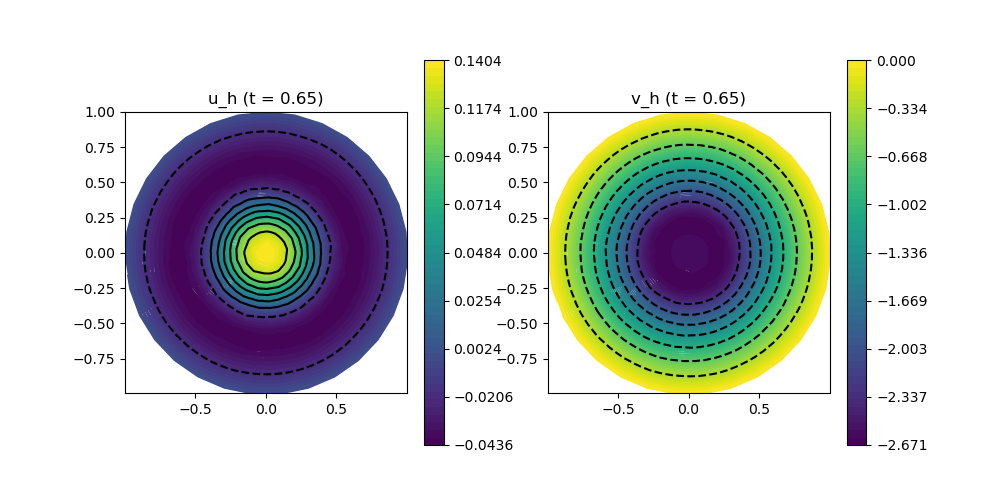
scalarplot!(p[1,1], xgrid, node_views[1], levels = 7, title = "u_h (t = $(Float64(sys.ctime)))")
scalarplot!(p[1,2], xgrid, node_views[2], levels = 7, title = "v_h (t = $(Float64(sys.ctime)))")
end
return nothing
end
# use time control solver by GradientRobustMultiPhysics
advance_until_time!(sys, timestep, T; do_after_each_timestep = do_after_each_timestep)
end
function grid_circle(center, radius, n; maxvol = 0.1)
builder=SimplexGridBuilder(Generator=Triangulate)
points = [point!(builder, center[1]+radius*sin(t),center[2]+radius*cos(t)) for t in range(0,2π,length=n)]
for i=1:n-1
facet!(builder,points[i],points[i+1])
end
facet!(builder,points[end],points[1])
simplexgrid(builder,maxvolume = maxvol)
end
endThis page was generated using Literate.jl.