A07 : Interpolation Between Meshes

(source code)

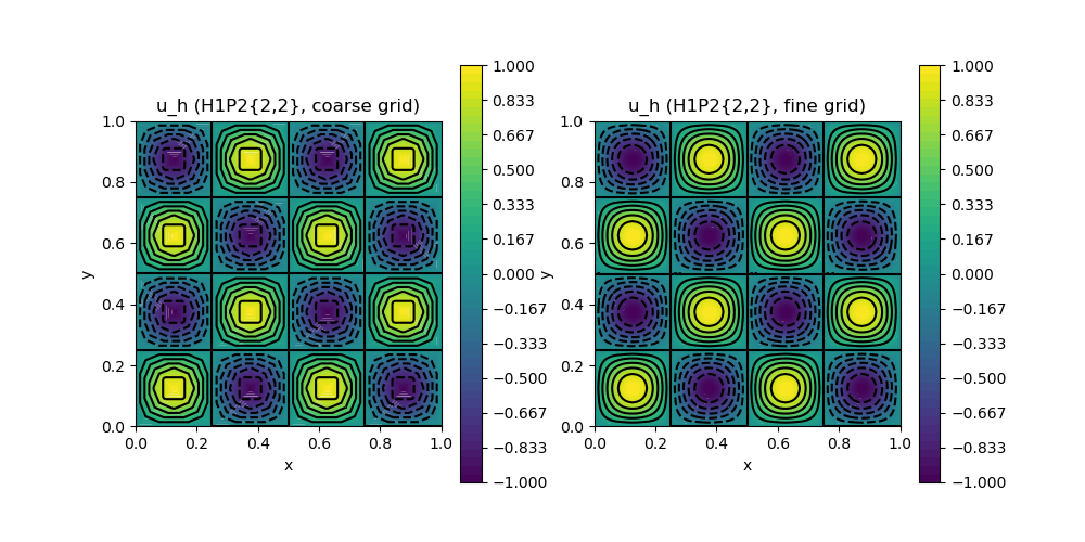
This example demonstrates the interpolation between meshes feature. Here, we interpolate a function withe the P2 element of a coarse triangulation and then interpolate this P2 function on two uniform refinements into some P1 function. Then, both finite element functions are plotted.

module ExampleA07_InterpolationBetweenMeshes

using GradientRobustMultiPhysics
using ExtendableGrids
using GridVisualize

# function to interpolate
function exact_u(result,x)
    result[1] = sin(4*pi*x[1])*sin(4*pi*x[2]);
    result[2] = cos(4*pi*x[1])*cos(4*pi*x[2]);
end
const u = DataFunction(exact_u, [2,2]; name = "u", dependencies = "X", bonus_quadorder = 5)

# everything is wrapped in a main function
function main(; ν = 1e-3, nrefinements = 4, verbosity = 0, Plotter = nothing)

    # set log level
    set_verbosity(verbosity)

    # generate two grids
    xgrid1 = uniform_refine(grid_unitsquare(Triangle2D),nrefinements)
    xgrid2 = uniform_refine(xgrid1, 2; store_parents = true)

    @show xgrid1 xgrid2

    # set finite element types for the two grids
    FEType1 = H1P2{2,2}
    FEType2 = H1P2{2,2}

    # generate coressponding finite element spaces and FEVectors
    FES1 = FESpace{FEType1}(xgrid1)
    FES2 = FESpace{FEType2}(xgrid2)
    FEFunction1 = FEVector(FES1)
    FEFunction2 = FEVector(FES2)

    # interpolate function onto first grid
    interpolate!(FEFunction1[1], u)

    # interpolate onto other grid
    @time interpolate!(FEFunction2[1], FEFunction1[1])
    @time interpolate!(FEFunction2[1], FEFunction1[1], use_cellparents = true)

    # plot
    p = GridVisualizer(; Plotter = Plotter, layout = (1,2), clear = true, resolution = (1000,500))
    scalarplot!(p[1,1], xgrid1, view(nodevalues(FEFunction1[1]),1,:), levels = 11, title = "u_h ($FEType1, coarse grid)")
    scalarplot!(p[1,2], xgrid2, view(nodevalues(FEFunction2[1]),1,:), levels = 11, title = "u_h ($FEType2, fine grid)")
end

end

This page was generated using Literate.jl.