215 : Two nonlinearly coupled PDEs (2D)
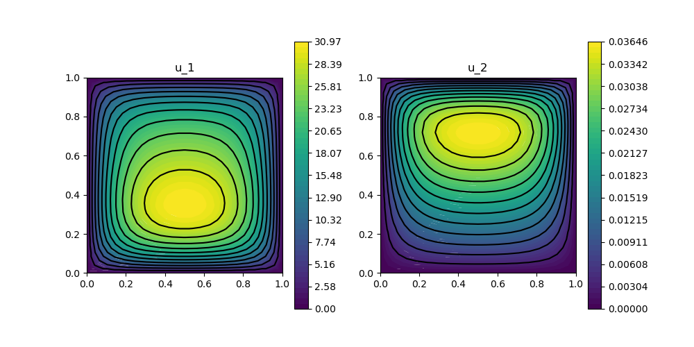
This example computes the solutions $u_1$ and $u_2$ of the two coupled nonlinear PDEs
\[\begin{aligned} -\nu_1 \Delta u_1 + \alpha_1 u_1u_2 & = f_1 \quad \text{in } \Omega\\ -\nu_2 \Delta u_2 + \alpha_2 u_1u_2 & = f_2 \quad \text{in } \Omega \end{aligned}\]
with given data $\nu$, $\alpha$ and right-hand sides $f_1$, $f_2$ on the unit cube domain $\Omega$.
This example demonstrates how to define this problem with one NonlinearForm per equation that can be automatically differentiated to solve the problem with Newton's method.
module Example215_TwoNonlinearCoupled2D

using GradientRobustMultiPhysics
using ExtendableGrids
using GridVisualize

# problem data
const f = [x -> 1, x -> 2*x[2]]
const ν = [1e-3,1]
const α = [1,1]

# everything is wrapped in a main function
function main(; verbosity = 0, Plotter = nothing)

    # set log level
    set_verbosity(verbosity)

    # build/load any grid (here: a uniform-refined 2D unit square into triangles)
    xgrid = uniform_refine(grid_unitsquare(Triangle2D),4)

    # create empty PDE description
    Problem = PDEDescription("Problem")

    # add two unknown with zero boundary data
    add_unknown!(Problem; unknown_name = "u", equation_name = "Equation for u")
    add_unknown!(Problem; unknown_name = "p", equation_name = "Equation for p")
    add_boundarydata!(Problem, 1, [1,2,3,4], HomogeneousDirichletBoundary)
    add_boundarydata!(Problem, 2, [1,2,3,4], HomogeneousDirichletBoundary)

    # add equations for unknowns as single NonlinearForms
    function operator_kernel(id)
        return function closure(result,input,x)
            # input = [u1,∇u1,u2]
            result[1] = α[id]*input[1]*input[4] - f[id](x)    # will be multiplied with identity of test function
            result[2] = ν[id]*input[2] # will be multiplied with 1st component of gradient of testfunction
            result[3] = ν[id]*input[3] # will be multiplied with 2nd component of gradient of testfunction
            return nothing
        end
    end
    add_operator!(Problem, 1, NonlinearForm(OperatorPair{Identity,Gradient}, [OperatorPair{Identity,Gradient},Identity], [1,2], operator_kernel(1), [3,4]; name = "ν1 (∇#1,∇#T) + α1 (#1 #2,#T) - (f1,#T)", dependencies = "X", newton = true))
    add_operator!(Problem, 2, NonlinearForm(OperatorPair{Identity,Gradient}, [OperatorPair{Identity,Gradient},Identity], [2,1], operator_kernel(2), [3,4]; name = "ν2 (∇#1,∇#T) + α2 (#1 #2,#T) - (f2,#T)", dependencies = "X", newton = true))

    # discretise (here: u1 with P3, u2 with P2)
    FETypes = [H1P3{1,2},H1P2{1,2}]
    FES = [FESpace{FETypes[1]}(xgrid),FESpace{FETypes[2]}(xgrid)]
    Solution = FEVector(FES)

    # show problem and Solution structure
    @show Problem Solution

    # solve for chosen Solution vector
    solve!(Solution, Problem; show_statistics = true)

    # plot solution (for e.g. Plotter = PyPlot)
    p = GridVisualizer(; Plotter = Plotter, layout = (1,2), clear = true, resolution = (1000,500))
    scalarplot!(p[1,1], xgrid, nodevalues_view(Solution[1])[1], levels = 11, title = "u_1")
    scalarplot!(p[1,2], xgrid, nodevalues_view(Solution[2])[1], levels = 11, title = "u_2")
end
end
This page was generated using Literate.jl.