202 : Linear Elasticity

(source code)

This example computes the solution $\mathbf{u}$ of the linear elasticity problem

\[\begin{aligned} -\mathrm{div} (\mathbb{C} \epsilon(\mathbf{u})) & = \mathbf{f} \quad \text{in } \Omega\\ \mathbb{C} \epsilon(\mathbf{u}) \cdot \mathbf{n} & = \mathbf{g} \quad \text{along } \Gamma_N \end{aligned}\]

with exterior force $\mathbf{f}$, Neumann boundary force $\mathbf{g}$, and the stiffness tensor

\[\mathbb{C} \epsilon(\mathbf{u}) = 2 \mu \epsilon( \mathbf{u}) + \lambda \mathrm{tr}(\epsilon( \mathbf{u}))\]

for isotropic media.

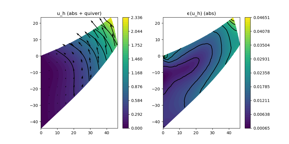
The domain will be the Cook membrane and the displacement has homogeneous boundary conditions on the left side of the domain and Neumann boundary conditions (i.e. a constant force that pulls the domain upwards) on the right side.

module Example202_LinearElasticity2D

using GradientRobustMultiPhysics
using ExtendableGrids
using GridVisualize

const g = DataFunction([0,10]; name = "g")

# everything is wrapped in a main function
function main(; verbosity = 0, E = 1000, ν = 0.4, Plotter = nothing)

    # set log level
    set_verbosity(verbosity)

    # load mesh and refine
    xgrid = simplexgrid("assets/2d_grid_cookmembrane.sg")
    xgrid = uniform_refine(xgrid,2)

    # compute Lame' coefficients from E and ν
    μ = (1/(1+ν))*E
    λ = (ν/(1-2*ν))*μ

    # PDE description via prototype and add data
    Problem = LinearElasticityProblem(2; shear_modulus = μ, lambda = λ)
    add_rhsdata!(Problem, 1, LinearForm(Identity, g; regions = [2], AT = ON_BFACES))
    add_boundarydata!(Problem, 1, [4], HomogeneousDirichletBoundary)

    # show and solve PDE
    @show Problem
    FEType = H1P1{2} # P1-Courant FEM will be used
    Solution = solve(Problem, FESpace{FEType}(xgrid))

    # plot stress on displaced mesh
    displace_mesh!(xgrid, Solution[1]; magnify = 4)
    p = GridVisualizer(; Plotter = Plotter, layout = (1,2), clear = true, resolution = (1000,500))
    scalarplot!(p[1,1], xgrid, view(nodevalues(Solution[1]; abs = true),1,:), levels = 7, title = "u_h")
    vectorplot!(p[1,1], xgrid, evaluate(PointEvaluator(Solution[1], Identity)), spacing = 5, clear = false, title = "u_h (abs + quiver)")
    scalarplot!(p[1,2], xgrid, view(nodevalues(Solution[1], SymmetricGradient{1/√2}; abs = true),1,:), levels = 7, title = "ϵ(u_h) (abs)")
end

end

This page was generated using Literate.jl.