A10 : Poisson-Problem with periodic boundary

(source code)

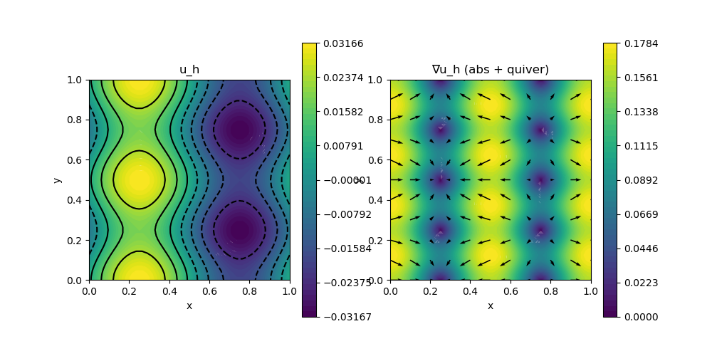
This example computes the solution $u$ of the Poisson problem

\[\begin{aligned} -\Delta u & = f \quad \text{in } \Omega \end{aligned}\]

with some right-hand side $f$ on the unit square (dim = 2) or cube (dim = 3) domain $\Omega$ with periodic boundary conditions in all directions. The 3D case only works for order = 1 and order = 2, order = 3 is work in progress.

module ExampleA10_PoissonPeriodic

using GradientRobustMultiPhysics
using ExtendableGrids
using GridVisualize

# right-hand side function
const f2D = DataFunction((result, x) -> (result[1] = sin(2*pi*x[1]) + cos(4*pi*x[2]);)
            ,[1,2]; dependencies = "X", name = "f", bonus_quadorder = 5)

const f3D = DataFunction((result, x) -> (result[1] = sin(2*pi*x[1]) + cos(4*pi*x[2]) + cos(2*pi*x[3]);)
             ,[1,3]; dependencies = "X", name = "f", bonus_quadorder = 5)

# everything is wrapped in a main function
function main(; verbosity = 0, μ = 1, order = 2, dim = 2, nrefinements = 5 - dim, Plotter = nothing)

    # set log level
    set_verbosity(verbosity)

    # build/load any grid (here: a uniform-refined 2D unit square into triangles)
    xgrid = uniform_refine(dim == 2 ? grid_unitsquare(Triangle2D) : grid_unitcube(Tetrahedron3D), nrefinements)

    # create empty PDE description
    Problem = PDEDescription("Poisson problem")

    # add unknown(s) (here: "u" that gets id 1 for later reference)
    add_unknown!(Problem; unknown_name = "u", equation_name = "Poisson equation")

    # add left-hand side PDEoperator(s) (here: only Laplacian)
    add_operator!(Problem, [1,1], LaplaceOperator(μ))

    # add right-hand side data (here: f = [1] in region(s) [1])
    add_rhsdata!(Problem, 1, LinearForm(Identity, dim == 2 ? f2D : f3D; regions = [1]))

    # discretise = choose FEVector with appropriate FESpaces
    if dim == 2
        FEType = H1Pk{1,2,order}
    else
        if order == 1
            FEType = H1P1{1}
        elseif order == 2
            FEType = H1P2{1,3}
        elseif order == 3
            FEType = H1P3{1,3}
        end
    end
    FES = FESpace{FEType}(xgrid)
    Solution = FEVector(FES)

    # add periodic boundary
    if dim == 2
        dofsX, dofsY = get_periodic_coupling_info(FES, xgrid, 2, 4, (f1,f2) -> abs(f1[2] - f2[2]) < 1e-14)
        add_constraint!(Problem, CombineDofs(1, 1, dofsX, dofsY))
        dofsX2, dofsY2 = get_periodic_coupling_info(FES, xgrid, 1, 3, (f1,f2) -> abs(f1[1] - f2[1]) < 1e-14)
        add_constraint!(Problem, CombineDofs(1, 1, dofsX2, dofsY2))
    elseif dim == 3
        #add_boundarydata!(Problem, 1, [1,2,3,4,5,6], HomogeneousDirichletBoundary)
        dofsX, dofsY = get_periodic_coupling_info(FES, xgrid, 2, 4, (f1,f2) -> abs(f1[1] - f2[1]) + abs(f1[3] - f2[3]) < 1e-14)
        add_constraint!(Problem, CombineDofs(1, 1, dofsX, dofsY))
        dofsX2, dofsY2 = get_periodic_coupling_info(FES, xgrid, 1, 6, (f1,f2) -> abs(f1[1] - f2[1]) + abs(f1[2] - f2[2]) < 1e-14)
        add_constraint!(Problem, CombineDofs(1, 1, dofsX2, dofsY2))
        dofsX3, dofsY3 = get_periodic_coupling_info(FES, xgrid, 3, 5, (f1,f2) -> abs(f1[3] - f2[3]) + abs(f1[2] - f2[2]) < 1e-14)
        add_constraint!(Problem, CombineDofs(1, 1, dofsX3, dofsY3))
    end

    # show problem and Solution structure
    @show Problem Solution

    # solve for chosen Solution vector
    solve!(Solution, Problem; show_statistics = true)

    # plot solution (for e.g. Plotter = PyPlot)
    p = GridVisualizer(; Plotter = Plotter, layout = (1,2), clear = true, resolution = (1000,500))
    gridplot!(p[1,1], xgrid)
    scalarplot!(p[1,2], xgrid, view(nodevalues(Solution[1]),1,:), levels = 7, title = "u_h")
end

end

This page was generated using Literate.jl.