220 : Planar Lattice Flow 2D
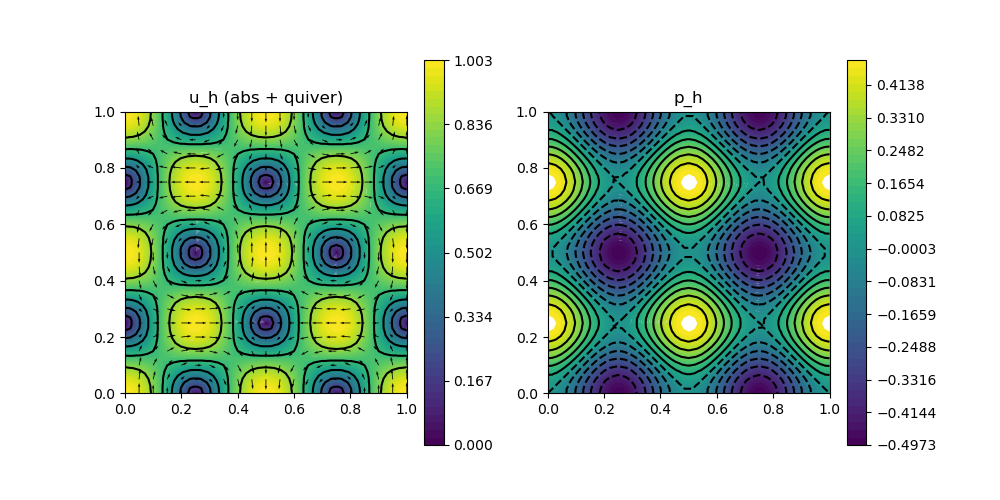
This example computes an approximation to the planar lattice flow test problem of the Stokes equations
\[\begin{aligned} - \nu \Delta \mathbf{u} + (\mathbf{u} \cdot \nabla) \mathbf{u} + \nabla p & = \mathbf{f}\\ \mathrm{div}(\mathbf{u}) & = 0 \end{aligned}\]
with an exterior force $\mathbf{f}$ and some viscosity parameter $\nu$ and Dirichlet boundary data for $\mathbf{u}$.
Here the exact data for the planar lattice flow
\[\begin{aligned} \mathbf{u}(x,y,t) & := \exp(-8 \pi^2 \nu t) \begin{pmatrix} \sin(2 \pi x) sin(2 \pi y) \\ \cos(2 \pi x) cos(2 \pi y) \end{pmatrix}\\ p(x,y,t) & := \exp(-8 \pi^2 \nu t) ( \cos(4 \pi x) - \cos(4 \pi y)) / 4 \end{aligned}\]
is prescribed at fixed time $t = 0$ with $\mathbf{f} = - \nu \Delta \mathbf{u}$.
In this example the Navier-Stokes equations are solved with a pressure-robust variant of the Bernardi–Raugel finite element method and the nonlinear convection term (that involves reconstruction operators) is automatically differentiated for a Newton iteration.
module Example220_PlanarLatticeFlow2D

using GradientRobustMultiPhysics
using ExtendableGrids
using GridVisualize

# everything is wrapped in a main function
function main(; ν = 2e-4, nrefinements = 5, verbosity = 0, Plotter = nothing)

    # set log level
    set_verbosity(verbosity)

    # generate a unit square mesh and refine
    xgrid = uniform_refine(grid_unitsquare(Triangle2D),nrefinements)

    # negotiate data
    u = DataFunction((result, x, t) -> (
            result[1] = exp(-8*pi*pi*ν*t)*sin(2*pi*x[1])*sin(2*pi*x[2]);
            result[2] = exp(-8*pi*pi*ν*t)*cos(2*pi*x[1])*cos(2*pi*x[2]);
        ), [2,2]; name = "u", dependencies = "XT", bonus_quadorder = 6)
    p = DataFunction((result, x, t) -> (
            result[1] = exp(-8*pi*pi*ν*t)*(cos(4*pi*x[1])-cos(4*pi*x[2])) / 4
        ), [1,2]; name = "p", dependencies = "XT", bonus_quadorder = 4)
    Δu = eval_Δ(u)
    f = DataFunction((result, x, t) -> (
            result .= -ν*Δu(x,t); # ∇p + (u ⋅ ∇)u = 0
        ), [2,2]; name = "f", dependencies = "XT", bonus_quadorder = 4)

    # set finite elements (Bernardi--Raugel)
    FEType = [H1BR{2}, L2P0{1}]

    # prepare comparison plot
    vis = GridVisualizer(; Plotter = Plotter, layout = (2,2), clear = true, resolution = (1000,1000))

    for probust in [false,true]

        # set identity operator
        IdentityV = probust ? ReconstructionIdentity{HDIVBDM1{2}} : Identity

        # setup a bestapproximation problem via a predefined prototype
        Problem = PDEDescription("planar lattice flow problem")
        add_unknown!(Problem; equation_name = "momentum equation", unknown_name = "velocity")
        add_unknown!(Problem; equation_name = "incompressibility constraint", unknown_name = "pressure")
        add_operator!(Problem, [1,1], LaplaceOperator(ν; store = true))
        add_operator!(Problem, [1,2], LagrangeMultiplier(Divergence))
        add_operator!(Problem, [1,1], ConvectionOperator(1, IdentityV, 2, 2; test_operator = IdentityV, newton = true))
        add_constraint!(Problem, FixedIntegralMean(2,0))
        add_boundarydata!(Problem, 1, [1,2,3,4], BestapproxDirichletBoundary; data = u)
        add_rhsdata!(Problem, 1, LinearForm(IdentityV, f))
        @show Problem

        # create finite element spaces and solve
        FES = [FESpace{FEType[1]}(xgrid),FESpace{FEType[2]}(xgrid)]
        Solution = FEVector(FES; name = ["u_h $(probust ? "(probust)" : "classical")", "p_h $(probust ? "(probust)" : "classical")"])
        solve!(Solution, Problem; show_statistics = true, show_solver_config = true)

        # calculate L2 errors for u and p
        L2errorV = L2ErrorIntegrator(u, Identity)
        L2errorP = L2ErrorIntegrator(p, Identity)
        println("|| u - u_h || = $(sqrt(evaluate(L2errorV,Solution[1])))")
        println("|| p - p_h || = $(sqrt(evaluate(L2errorP,Solution[2])))")

        # plot
        scalarplot!(vis[1+probust,1],xgrid,view(nodevalues(Solution[1]; abs = true),1,:), levels = 5, title = "$(Solution[1].name) (abs + quiver)")
        vectorplot!(vis[1+probust,1],xgrid,evaluate(PointEvaluator(Solution[1], Identity)), spacing = 0.05, clear = false)
        scalarplot!(vis[1+probust,2],xgrid,view(nodevalues(Solution[2]),1,:), levels = 7, title = "$(Solution[2].name)")
    end
end

end
This page was generated using Literate.jl.