240 : Compressible Stokes 2D

(source code)

This example solves the compressible Stokes equations where one seeks a (vector-valued) velocity $\mathbf{u}$, a density $\varrho$ and a pressure $p$ such that

\[\begin{aligned} - \mu \Delta \mathbf{u} + \lambda \nabla(\mathrm{div}(\mathbf{u})) + \nabla p & = \mathbf{f} + \varrho \mathbf{g}\\ \mathrm{div}(\varrho \mathbf{u}) & = 0\\ p & = eos(\varrho)\\ \int_\Omega \varrho \, dx & = M\\ \varrho & \geq 0. \end{aligned}\]

Here eos $eos$ is some equation of state function that describes the dependence of the pressure on the density (and further physical quantities like temperature in a more general setting). Moreover, $\mu$ and $\lambda$ are Lame parameters and $\mathbf{f}$ and $\mathbf{g}$ are given right-hand side data.

In this example we solve a analytical toy problem with the prescribed solution

\[\begin{aligned} \mathbf{u}(\mathbf{x}) & =0\\ \varrho(\mathbf{x}) & = 1 - (x_2 - 0.5)/c\\ p &= eos(\varrho) := c \varrho^\gamma \end{aligned}\]

such that $\mathbf{f} = 0$ and $\mathbf{g}$ nonzero to match the prescribed solution.

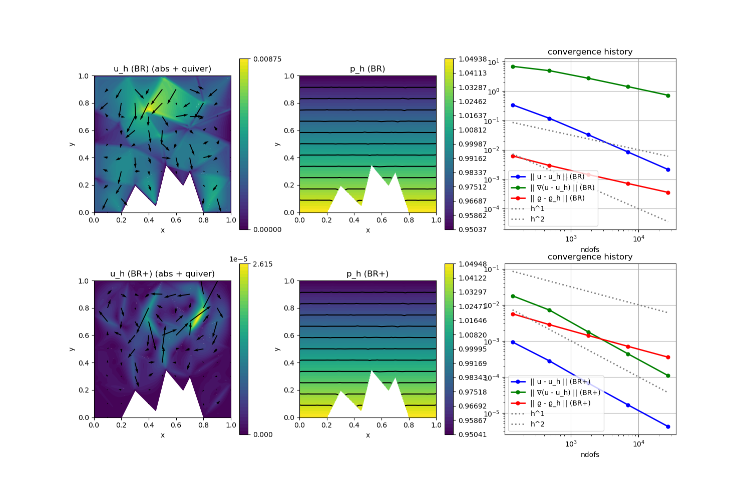
This example is designed to study the well-balanced property of a discretisation. The gradient-robust discretisation approximates the well-balanced state much better, i.e. has a much smaller L2 velocity error. For larger c the problem gets more incompressible which reduces the error further as then the right-hand side is a perfect gradient also when evaluated with the (now closer to a constant) discrete density. See reference below for more details.

module Example240_CompressibleStokes2D

using GradientRobustMultiPhysics
using ExtendableGrids
using GridVisualize

# parameters
const c = 10
const γ = 1
const μ = 1e-3
const λ = -2/3*μ

# the equation of state
const equation_of_state = DataFunction((p, ϱ) -> p[1] = c.*ϱ[1].^γ, [1,1])

# data for exact solution u = 0 and ϱ = ϱ
const ϱ = DataFunction((result,x) -> (result[1] = (1.0 - (x[2] - 0.5)/c)), [1,2]; name = "ϱ", dependencies = "X", bonus_quadorder = 2)
const g = DataFunction((result,x) -> (result[2] = - (1.0 - (x[2] - 0.5)/c)^(γ-2) * γ), [2,2]; name = "g", dependencies = "X", bonus_quadorder = 4)
const f = DataFunction((result,x) -> (result[2] = result[2] = - (1.0 - (x[2] - 0.5)/c)^(γ-1) * γ), [2,2]; name = "f", dependencies = "X", bonus_quadorder = 4)

# everything is wrapped in a main function
function main(; use_gravity = true, newton = false, nlevels = 4, Plotter = nothing, verbosity = 0)

    # set log level
    set_verbosity(verbosity)

    # load mesh and compute mass of exact ϱ
    xgrid = simplexgrid("assets/2d_mountainrange.sg")
    M = integrate(xgrid, ON_CELLS, ϱ, 1)

    # prepare error calculation
    VeloError = L2NormIntegrator(2, Identity)
    VeloGradError = L2NormIntegrator(4, Gradient)
    DensityError = L2ErrorIntegrator(ϱ, Identity; quadorder = 2)
    Results = zeros(Float64,6,nlevels)
    NDoFs = zeros(Int,nlevels)

    # set finite element types [velocity, density,  pressure]
    FETypes = [H1BR{2}, L2P0{1}] # Bernardi--Raugel x P0

    # solve
    Solution = [nothing, nothing]
    for lvl = 1 : nlevels
        if lvl > 1
            xgrid = uniform_refine(xgrid)
        end

        # generate FESpaces and solution vector
        FES = [FESpace{FETypes[1]}(xgrid), FESpace{FETypes[2]}(xgrid)]
        Solution = [FEVector(FES),FEVector(FES)]
        NDoFs[lvl] = length(Solution[1].entries)

        # solve with and without reconstruction
        for reconstruct in [true, false]
            Target = Solution[reconstruct+1]
            setup_and_solve!(Target, xgrid; use_gravity = use_gravity, reconstruct = reconstruct, newton = newton, c = c, M = M, λ = λ, μ = μ, γ = γ)
            Results[reconstruct ? 2 : 1, lvl] = sqrt(evaluate(VeloError,Target[1]))
            Results[reconstruct ? 4 : 3, lvl] = sqrt(evaluate(VeloGradError,Target[1]))
            Results[reconstruct ? 6 : 5, lvl] = sqrt(evaluate(DensityError,Target[2]))

            # check error in mass constraint
            Md = sum(Target[2][:] .* xgrid[CellVolumes])
            println("\tmass_error = $M - $Md = $(abs(M-Md))")
        end
    end

    # print convergence history tables
    print_convergencehistory(NDoFs, Results[1:2,:]'; X_to_h = X -> X.^(-1/2), ylabels = ["||u-u_h|| (BR)","||u-u_h|| (BR+)"], xlabel = "ndof")
    print_convergencehistory(NDoFs, Results[3:4,:]'; X_to_h = X -> X.^(-1/2), ylabels = ["||∇(u-u_h)|| (BR)","||∇(u-u_h)|| (BR+)"], xlabel = "ndof")
    print_convergencehistory(NDoFs, Results[5:6,:]'; X_to_h = X -> X.^(-1/2), ylabels = ["||ϱ-ϱ_h|| (BR)","||ϱ-ϱ_h|| (BR+)"], xlabel = "ndof")

    # plot everything
    p = GridVisualizer(; Plotter = Plotter, layout = (2,3), clear = true, resolution = (1500,1000))
    scalarplot!(p[1,1],xgrid,view(nodevalues(Solution[1][1]; abs = true),1,:), levels = 0, title = "u_h (BR) (abs + quiver)")
    vectorplot!(p[1,1],xgrid,evaluate(PointEvaluator(Solution[1][1], Identity)), spacing = 0.1, clear = false)
    scalarplot!(p[1,2],xgrid,view(nodevalues(Solution[1][2]),1,:), levels = 11, title = "p_h (BR)")
    scalarplot!(p[2,1],xgrid,view(nodevalues(Solution[2][1]; abs = true),1,:), levels = 0, title = "u_h (BR+) (abs + quiver)")
    vectorplot!(p[2,1],xgrid,evaluate(PointEvaluator(Solution[2][1], Identity)), spacing = 0.1, clear = false)
    scalarplot!(p[2,2],xgrid,view(nodevalues(Solution[2][2]),1,:), levels = 11, title = "p_h (BR+)")
    convergencehistory!(p[1,3], NDoFs, Results[[1,3,5],:]'; add_h_powers = [1,2], X_to_h = X -> X.^(-1/2), ylabels = ["|| u - u_h || (BR)", "|| ∇(u - u_h) || (BR)", "|| ϱ - ϱ_h || (BR)"], legend = :lb)
    convergencehistory!(p[2,3], NDoFs, Results[[2,4,6],:]'; add_h_powers = [1,2], X_to_h = X -> X.^(-1/2), ylabels = ["|| u - u_h || (BR+)", "|| ∇(u - u_h) || (BR+)", "|| ϱ - ϱ_h || (BR+)"], legend = :lb)
end

function setup_and_solve!(Solution, xgrid;
    c = 1, γ = 1, M = 1, μ = 1, λ = 0,
    use_gravity = true,
    reconstruct = true,
    newton = true)

    # generate empty PDEDescription for three unknowns (u, ϱ. p)
    Problem = PDEDescription("compressible Stokes problem")
    add_unknown!(Problem; unknown_name = "v", equation_name = "momentum equation")
    add_unknown!(Problem; unknown_name = "ϱ", equation_name = "continuity equation")
    add_boundarydata!(Problem, 1,  [1,2,3,4], HomogeneousDirichletBoundary)

    # momentum equation
    hdiv_space = HDIVBDM1{2} # HDIVRT0{2} also works
    VeloIdentity = reconstruct ? ReconstructionIdentity{hdiv_space} : Identity
    VeloDivergence = reconstruct ? ReconstructionDivergence{hdiv_space} : Divergence
    add_operator!(Problem, [1,1], LaplaceOperator(2*μ; store = true))
    if λ != 0
        add_operator!(Problem, [1,1], BilinearForm([VeloDivergence,VeloDivergence]; name = "λ (div(u),div(v))", factor = λ, store = true))
    end

    # add pressure term -(div(v),p(ϱ))
	add_operator!(Problem, [1,2], BilinearForm([VeloDivergence, Identity], feval_action(equation_of_state); factor = -1, name = "-(div v, eos(ϱ))", apply_action_to = [2], store = true))

    # add gravity either as usual or as explicit right-hand side force
    if use_gravity
        add_operator!(Problem, [1,2], BilinearForm([VeloIdentity,Identity], fdotv_action(g); factor = -1, name = "(g ⋅ v) ϱ", store = true))
    else
        # exact gravity term for right-hand side
        add_rhsdata!(Problem, 1, LinearForm(VeloIdentity, f; store = true))
    end

    # initial values for density (constant)
    fill!(Solution[2], M/sum(xgrid[CellVolumes]))

    # solve
    if newton
        # add upwinded continuity equation as NonlinearForm
        function upwind_kernel(result, input, face)
            # input = [NormalFlux, Identity on parent 1, Identity on parent 2]
            if input[1] > 0
                result[1] = input[1] * input[2]
            else
                result[1] = input[1] * input[3]
            end
        end
        add_operator!(Problem, 2, NonlinearForm(Jump(Identity), [NormalFlux,Parent{1}(Identity),Parent{2}(Identity)], [1,2,2], upwind_kernel, [1,3]; dependencies = "I", AT = ON_IFACES, sparse_jacobian = false, name = "(div_upw(ϱ_hu_h),q_h)"))

        # add mass constraint on density and solve
        add_constraint!(Problem, FixedIntegralMean(2, M/sum(xgrid[CellVolumes])))
        solve!(Solution, Problem; maxiterations = 20)
    else
        # add continuity equation as linear operator and solve by pseudo timestepping
        add_operator!(Problem, [2,2], FVConvectionDiffusionOperator(1))
        # time-dependent solver with three equations [1] velocity, [2] density
        # solved iteratively [1] => [2] in each pseudo time step until stationarity
        TCS = TimeControlSolver(Problem, Solution, BackwardEuler;
                                            subiterations = [[1],[2]], # solve [1], then [2]
                                            skip_update = [-1,1], # only matrix of eq [2] changes
                                            timedependent_equations = [2], # only eq [2] is time-dependent
                                            maxiterations = 1,
                                            check_nonlinear_residual = false,
                                            show_iteration_details = false)
        timestep = 2 * μ / (M*c)
        maxtimesteps = 500
        stationarity_threshold = c*1e-14/μ
        advance_until_stationarity!(TCS, timestep; maxtimesteps = maxtimesteps, stationarity_threshold = stationarity_threshold)
    end
end
end

This page was generated using Literate.jl.